wages |>
  ggplot(aes(x = height, y = log(income))) +
geom_point(alpha = 0.1)Models
Your Turn 1
- Change the working directory to the folder where
wages.xlsxis located and this file is saved. - Then import
wages.xlsxas wages and copy the code to your setup chunk. - Be sure to set
NA:toNA. - Switch the
evaloption in the YAML header totrue.
Your Turn 2
- Fit the model
\[ \log(\text{income}) = \beta_0 + \beta_1 \cdot \text{education} + \epsilon \]
- Store the result in an object called
mod_e. - Examine the output. What does it look like?
Your Turn 3
Use a pipe to model log(income) against height. Then use broom and dplyr functions to extract:
- The coefficient estimates and their related statistics
- The adj.r.squared and p.value for the overall model
Your Turn 4
Model log(income) against education and height and sex. Can you interpret the coefficients?
Your Turn 5
Add + geom_smooth(method = lm) to the code below. What happens?
Your Turn 6
Use add_predictions() to make the plot below. Facetting is by level of education.
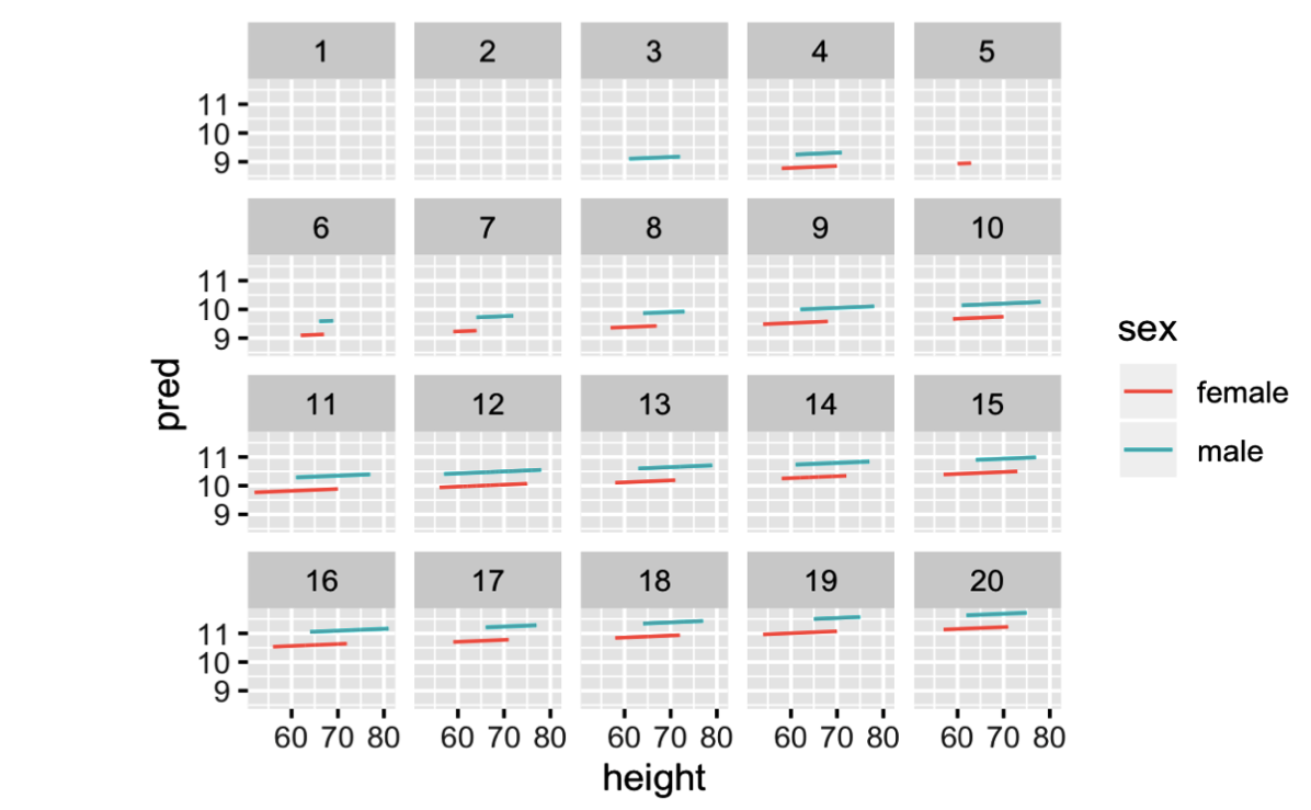
# In case you haven't made the ehs model
mod_ehs <- wages|>
  lm(log(income) ~ education + height + sex, data = _)

# Make plot here
Your Turn 7
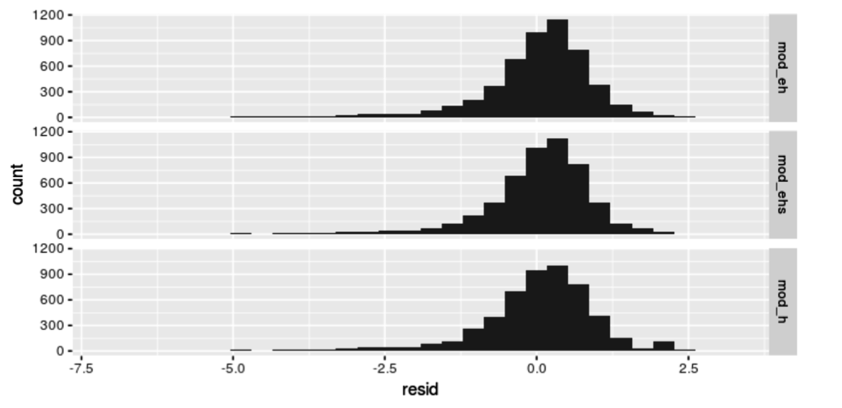
Use gather_residuals() to make the plot below.
Caution
Models mod_h and mod_ehs should be available in your environment because you fitted them in previous sections. But you have to fit and store the model mod_eh which stands for education and height.
# Make the plot hereTake Aways
Use
glance(),tidy(), andaugment()from the broom package to return model values in a data frame.Use
add_predictions()orgather_predictions()orspread_predictions()from the modelr package to visualize predictions.Use
add_residuals()orgather_residuals()orspread_residuals()from the modelr package to visualize residuals.