Hypothesis Testing
Statistical Framework
General data modeling framework
- You have some data \(\{x_1, \dots, x_n\}\) that you presume have been sampled independently from their corresponding random variables \(\{X_1, \dots, X_n\}\);
- You formulate a simple hypothesis \(H_0\), called null hypothesis, about the distribution from which this data were sampled;
- You want to confront this hypothesis against an alternative hypothesis \(H_a\) using your finite amount of data;
- You use a test statistic \(T(X_1, \dots, X_n)\) that depends on the sample (and thus that you can calculate anytime you observe a sample) and of which you know (an approximation of) the distribution when you assume that your null hypothesis is true; it is called the null distribution of the test statistic \(T\);
- You compute the value \(t_0\) of this test statistic with your observed data;
- You strongly reject \(H_0\) if \(t_0\) falls on the tails of the null distribution of \(T\); or,
- You lack evidence to reject \(H_0\) if \(t_0\) ends up in the central part of the null distribution of \(T\).
- Warning: It is straightforward from this setup to understand that the problem is not symmetric in the hypotheses. Indeed, the procedure relies on what happens when \(H_0\) is true but does not depend on \(H_a\).
Test Statistic
Theoretical aspects
You design a test statistic \(T(X_1, \dots, X_n)\) for the purpose of performing this test which must satisfy at least the first three of the following four properties:
- It evaluates to real values;
- You have all the required knowledge to compute its value once you observe the data;
- If \(H_0\) is true, then small values of the statistic should comfort you with the idea that \(H_0\) is a reasonable assumption, while larger values of the statistic should generate suspicion about \(H_0\) in favor of the alternative hypothesis \(H_a\);
- [optional] If \(H_0\) is true, then it can be very helpful to have access to the (asymptotic) distribution of the test statistic under classical assumptions (such as normality).
Example: Test on the mean
Suppose you have a sample of \(n\) i.i.d. random variables \(X_1, \dots, X_n \sim \mathcal{N}(\mu, \sigma^2)\) and you know the value of \(\sigma^2\). We want to test whether the mean \(\mu\) of the distribution is equal to some pre-specified value \(\mu_0\). We can therefore use \(H_0: \mu = \mu_0\) vs. \(H_a: \mu \ne \mu_0\). At this point, a good candidate test statistic to look at for performing this test is: \[ T(X_1, \dots, X_n) := \sqrt{n} \frac{\overline X - \mu_0}{\sigma}, \quad \mbox{with} \quad \overline X := \frac{1}{n} \sum_{i=1}^n X_i. \]
- It evaluates to real values;
- You have all the required knowledge to compute its value once you observe the data (\(\overline x\));
- The sample mean \(\overline X\) is an unbiased estimator of the true unknown mean \(\mu\); so, if \(H_0\) is true, then \(\overline X\) will produce values that are close to \(\mu_0\); hence, small values of \(T\) will comfort you with the idea that \(H_0\) is a reasonable assumption, while larger values, both positive or negative, of the statistic should generate suspicion about \(H_0\) in favor of the alternative hypothesis \(H_a\);
- If you assume normality and independence of the sample, then \(T \sim \mathcal{N}(0, 1)\) under \(H_0\).
Distribution of the test statistic under \(H_0\)
Parametric testing. If you designed your test statistic carefully, you might have access to its theoretical distribution when \(H_0\) is true under distributional assumptions about the data. This is called parametric hypothesis testing.
Asymptotic testing. If it is not the case, you can often derive the theoretical distribution of the statistic under the null hypothesis asymptotically, i.e. assuming that you have a large sample (\(n \gg 1\)); this is called asymptotic hypothesis testing.
Bootstrap testing. If you are in a large sample size regime but still cannot have access to the theoretical distribution of your test statistic, you can approach this distribution using bootstrapping; this is called bootstrap hypothesis testing.
Permutation testing. If you are in a low sample size regime, then you can approach the distribution of the test statistic using permutations; this is called permutation hypothesis testing.
Two-sided vs. one-sided hypothesis tests
Depending on what you put into the alternative hypothesis \(H_a\), larger values of the test statistic that raise suspicion regarding the validity of \(H_0\) might mean:
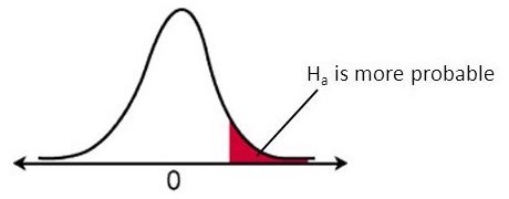
- larger values only on the right tail of the null distribution of \(T\);
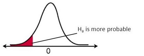
- larger values only on the left tail of the null distribution of \(T\);
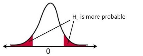
- larger values on both tails.
In the first two cases, we say that the test is one-sided. In the latter case, we say that the test is two-sided because we interpret large values in both tails as suspicious.
Example: Test on the mean (continued)
Suppose you have a sample of \(n\) i.i.d. random variables \(X_1, \dots, X_n \sim \mathcal{N}(\mu, \sigma^2)\) and you know the value of \(\sigma^2\). We want to test whether the mean \(\mu\) of the distribution is equal to some pre-specified value \(\mu_0\). As we have seen, a good candidate test statistic to look at for performing this test is:
\[ T(X_1, \dots, X_n) := \sqrt{n} \frac{\overline X - \mu_0}{\sigma}, \quad \mbox{with} \quad \overline X := \frac{1}{n} \sum_{i=1}^n X_i. \]
Now, using this test statistic, we might be interested in performing three different tests:
- \(H_0: \mu = \mu_0\) vs. \(H_a: \mu > \mu_0\);
- \(H_0: \mu = \mu_0\) vs. \(H_a: \mu < \mu_0\);
- \(H_0: \mu = \mu_0\) vs. \(H_a: \mu \ne \mu_0\).
\(H_0: \mu = \mu_0\) vs. \(H_a: \mu > \mu_0\)
\[ T(X_1, \dots, X_n) := \sqrt{n} \frac{\overline X - \mu_0}{\sigma} \] Remember that we must look at large values of \(T\) that raise suspicion in favor of \(H_a\).
\(\overline X\) is an unbiased estimator of the true mean.
Large negative values of \(T\) that happen when the true mean is far less than \(\mu_0\) does not raise suspicion in favor of \(H_a\).
Large positive values of \(T\) that happen when the true mean is far more than \(\mu_0\) does raise suspicion in favor of \(H_a\).
Conclusion: we are interested only in the right tail of the null distribution of \(T\) to find evidence to reject \(H_0\).
\(H_0: \mu = \mu_0\) vs. \(H_a: \mu < \mu_0\)
\[ T(X_1, \dots, X_n) := \sqrt{n} \frac{\overline X - \mu_0}{\sigma} \] Remember that we must look at large values of \(T\) that raise suspicion in favor of \(H_a\).
\(\overline X\) is an unbiased estimator of the true mean.
Large negative values of \(T\) that happen when the true mean is far more than \(\mu_0\) does not raise suspicion in favor of \(H_a\).
Large positive values of \(T\) that happen when the true mean is far less than \(\mu_0\) does raise suspicion in favor of \(H_a\).
Conclusion: we are interested only in the left tail of the null distribution of \(T\) to find evidence to reject \(H_0\).
\(H_0: \mu = \mu_0\) vs. \(H_a: \mu \ne \mu_0\)
\[ T(X_1, \dots, X_n) := \sqrt{n} \frac{\overline X - \mu_0}{\sigma} \] Remember that we must look at large values of \(T\) that raise suspicion in favor of \(H_a\).
\(\overline X\) is an unbiased estimator of the true mean.
Large negative values of \(T\) that happen when the true mean is far more than \(\mu_0\) does raise suspicion in favor of \(H_a\).
Large positive values of \(T\) that happen when the true mean is far less than \(\mu_0\) does raise suspicion in favor of \(H_a\).
Conclusion: we are interested in both the left and the right tails of the null distribution of \(T\) to find evidence to reject \(H_0\).
Making a decision
Type I and Type II errors
So we are now at a point where we know which tail(s) which we should look at and we now need to make a decision as to what large means. In other words, above which threshold on all possible values of my test statistic should I consider that I can reject \(H_0\).
- Notice that you are going to take this decision based on the null distribution.
- When you decide to reject or not, you might make an error:
| Decision | \(H_0\) is true | \(H_a\) is true |
|---|---|---|
| Do not reject \(H_0\) | Well done | Type II error |
| Reject \(H_0\) | Type I error | Well done |
- The only error rate you can control is the type I error rate because it is a probability computed assuming that the null hypothesis is true, which is exactly the situation we put ourselves in for making the decision (i.e. looking at the tails of the null distribution of \(T\)).
Significance level
At this point, you can decide that you do not want to make more than a certain amount of type I errors. So you want to force that \(\mathbb{P}_{H_0}(\mbox{reject } H_0) \le \alpha\), for some upper bound threshold \(\alpha\) on the probability of type I errors. This threshold is called significance level of the test and is often denoted by the greek letter \(\alpha\).
Let us now translate what this rule implies for the right-tail alternative case. The event “\(\mbox{reject } H_0\)” translates in this case into \(T > x\) for some \(x\) value of the test statistic \(T\). Hence, the rule becomes: \[ \mathbb{P}_{H_0}(T > x) \le \alpha \\ \Leftrightarrow 1 - \mathbb{P}_{H_0}(T \le x) \le \alpha \\ \Leftrightarrow 1 - F_T^{\left(H_0\right)}(x) \le \alpha \\ \Leftrightarrow F_T^{\left(H_0\right)}(x) \ge 1 - \alpha \] verified for all \(x \ge q_{1-\alpha}\), where \(q_{1-\alpha}\) is the quantile of order \(1-\alpha\) of the null distribution of \(T\).
Significance level (continued)
Decision-making rule:
- We reject \(H_0\) if the value \(t_0\) of the test statistic computed on the observed sample is greater than the quantile of order \(1-\alpha\) of the null distribution of \(T\);
- We decide that we lack evidence to reject \(H_0\) if the value \(t_0\) of the test statistic calculated on the observed sample is smaller than the quantile of order \(1-\alpha\) of the null distribution of \(T\).
- This decision-making rule guarantees that the probability of making a type I error is upper-bounded by the significance level \(\alpha\).
p-value
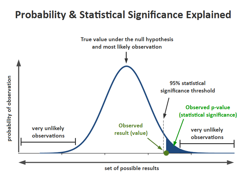
Definition. The p-value is a scalar value between \(0\) and \(1\) that measures what was the probability, assuming that the null hypothesis \(H_0\) is true, of observing the data we did observe, or data even more in favor of the alternative hypothesis.
Mathematical expression. If \(t_0\) is the value of the test statistic computed from the observed sample, then:
- \(p = \mathbb{P}_{H_0}(T > t_0)\) for right-tail hypothesis tests (e.g. \(H_a: \mu > \mu_0\) when testing the mean);
- \(p = \mathbb{P}_{H_0}(T < t_0)\) for left-tail hypothesis tests (e.g. \(H_a: \mu < \mu_0\) when testing the mean);
- \(p = 2 \min\left( \mathbb{P}_{H_0} \left( T > t_0 \right), \mathbb{P}_{H_0} \left( T < t_0 \right) \right)\) for two-tail hypothesis tests (e.g. \(H_a: \mu \ne \mu_0\) when testing the mean).
Interpretation. If the \(p\)-value is very small, it means that
- either we observed a miracle,
- or the null hypothesis might be wrong.
Decision-making rule. We can show that rejecting the null hypothesis when \(p \le \alpha\) also produces a decision-making rule that guarantees a probability of type I error at most \(\alpha\).
Decision-Making: Summary (right-tail scenario)
Statistical power of a test
Definition. It is the probability of correctly rejecting the null hypothesis, i.e. to reject it when the alternative is in fact correct. It is often denoted by \(\mu\). In terms of events, it is defined by: \[ \mu := \mathbb{P}_{H_a}(\mbox{Reject } H_0). \]
Usage. The statistical power of a test is an important aspect of the test because:
- it is an important performance indicator to compare different testing procedures (observe that there is not a unique statistic to perform a given test);
- it is often used in clinical trials or other types of trials (e.g. crash tests) to calibrate the number of observations required to achieve a given statistical power.
Remarks.
- The statistical power \(\mu\) is equal to \(1 - \beta\), where \(\beta\) is the greek letter often used to designate the probability of type II errors, \(\beta := \mathbb{P}_{H_a}(\mbox{Do not reject } H_0)\).
- Power calculations are difficult because it requires to put ourselves under \(H_a\), which is often of the form \(\mu > \mu_0\) or \(\mu < \mu_0\) or \(\mu \ne \mu_0\). In other words, you often lack information to compute probabilities assuming that the alternative hypothesis is true. You have to assess how the power changes as you explore different alternatives.
Compliance testing
Compliance testing aims at determining whether a process, product, or service complies with the requirements of a specification, technical standard, contract, or regulation.
Testing the mean
- Model. Let \((X_1, \dots, X_n)\) be \(n\) i.i.d. random variables that follow a normal distribution \(\mathcal{N}(\mu, \sigma^2)\).
- Hypotheses. \[ H_0: \mu = \mu_0 \quad \mbox{vs.} \quad H_a: \mu \ne \mu_0 \quad \mbox{or} \quad H_a: \mu > \mu_0 \quad \mbox{or} \quad H_a: \mu < \mu_0. \]
- Test Statistic. \[ Z_n = \sqrt{n} \frac{\overline X_n - \mu_0}{\sigma}. \]
- Problem. Under the null hypothesis, I do not have complete knowledge to compute the test statistic because I do not know the value of \(\sigma\).
Testing the mean with known variance
- Problem solved. I now have complete knowledge to compute the test statistic.
- Null distribution. The null distribution is \[ Z_n \stackrel{H_0}{\sim} \mathcal{N}(0, 1). \]
- R function. None
Testing the mean with unknown variance
- Problem solved. I plug in the empirical standard deviation instead of \(\sigma\) in the definition of the test statistic.
- Test Statistic. \[ T_n = \frac{\overline X_n - \mu_0}{\sqrt{\frac{S_{n-1}^2}{n}}}, \quad \mbox{with} \quad S_{n-1}^2 := \frac{1}{n-1} \sum_{i = 1}^n (X_i - \overline X)^2. \]
- Null distribution. \[ T_n \stackrel{H_0}{\sim} \mathcal{S}tudent(n-1). \]
- R function. t.test()
Testing the variance
- Assumptions. Let \((X_1, \dots, X_n)\) be \(n\) i.i.d. random variables that follow a normal distribution \(\mathcal{N}(\mu, \sigma^2)\).
- Hypotheses. \[ H_0: \sigma^2 = \sigma_0^2 \quad \mbox{vs.} \quad H_a: \sigma^2 \ne \sigma_0^2 \quad \mbox{or} \quad H_a: \sigma^2 > \sigma_0^2 \quad \mbox{or} \quad H_a: \sigma^2 < \sigma_0^2. \]
- Test Statistic. \[ U_n = \sum_{i = 1}^n \frac{(X_i - \mu)^2}{\sigma_0^2}. \]
- Problem. Under the null hypothesis, I do not have complete knowledge to compute the test statistic because I do not know the value of \(\mu\).
Testing the variance with known mean
- Problem solved. I now have complete knowledge to compute the test statistic.
- Null distribution. The null distribution is \[ U_n \stackrel{H_0}{\sim} \chi^2(n). \]
- R function. None.
Testing the variance with unknown mean
- Problem solved. I plug in the empirical mean instead of \(\mu\) in the definition of the test statistic.
- Test Statistic. \[ U_{n-1} = \sum_{i = 1}^n \frac{\left( X_i - \overline X_n \right)^2}{\sigma_0^2}. \]
- Null distribution. \[ U_{n-1} \stackrel{H_0}{\sim} \chi^2(n-1). \]
- R function. None.
Testing a proportion
Here we want to test whether the proportion \(p\) of individuals in a given population who have a feature of interest is equal to a pre-specified rate.
- Model. Let \((X_1, \dots, X_n)\) be \(n\) i.i.d. random variables that follow a Bernoulli distribution \(\mathcal{B}e(p)\). The interpretation is that \(X_i\) measures if individual \(i\) possesses the characteristic of which we want to know the proportion or not.
- Hypotheses. \[ H_0: p = p_0 \quad \mbox{vs.} \quad H_a: p \ne p_0 \quad \mbox{or} \quad H_a: p > p_0 \quad \mbox{or} \quad H_a: p < p_0. \]
- Test Statistic. \[ B_n = \sum_{i=1}^n X_i \]
- Null distribution. \[ B_n \sim \mathcal{B}inom(n,p_0) \]
- R function. binom.test()
Two-Sample Testing
Hypothesis tests for comparing the distributions that generated two independent samples.
Testing for variance differences
- Model. Let \((X_1, \dots, X_{n_x})\) be \(n_X\) i.i.d. random variables that follow a normal distribution \(\mathcal{N}(\mu_X, \sigma_X^2)\) and \((Y_1, \dots, Y_{n_Y})\) be \(n_Y\) i.i.d. random variables that follow a normal distribution \(\mathcal{N}(\mu_Y, \sigma_Y^2)\). Assume furthermore that the two samples are statistically independent.
- Hypotheses. \[ H_0: \sigma_X^2 = \sigma_Y^2 \quad \mbox{vs.} \quad H_a: \sigma_X^2 \ne \sigma_Y^2 \quad \mbox{or} \quad H_a: \sigma_X^2 > \sigma_Y^2 \quad \mbox{or} \quad H_a: \sigma_X^2 < \sigma_Y^2 \]
- Test Statistic. \[ V_n = \frac{S_X^2}{S_Y^2}, \quad \mbox{with} \quad S_X^2 = \frac{1}{n_X - 1} \sum_{i = 1}^{n_X} (X_i - \overline X_n)^2 \quad \mbox{and} \quad S_Y^2 = \frac{1}{n_Y - 1} \sum_{i = 1}^{n_Y} (Y_i - \overline Y_n)^2 \]
- Null distribution. \[ V_n \stackrel{H_0}{\sim} \mathcal{F}isher(n_X - 1, n_Y - 1) \]
- R function. var.test()
- Validity. Relies on the normality assumption and independence within and between samples.
Testing for mean differences
- Model. Let \((X_1, \dots, X_{n_x})\) be \(n_X\) i.i.d. random variables that follow a normal distribution \(\mathcal{N}(\mu_X, \sigma_X^2)\) and \((Y_1, \dots, Y_{n_Y})\) be \(n_Y\) i.i.d. random variables that follow a normal distribution \(\mathcal{N}(\mu_Y, \sigma_Y^2)\). Assume furthermore that the two samples are statistically independent.
- Hypotheses. \[ H_0: \mu_X = \mu_Y \quad \mbox{vs.} \quad H_a: \mu_X \ne \mu_Y \quad \mbox{or} \quad H_a: \mu_X > \mu_Y \quad \mbox{or} \quad H_a: \mu_X < \mu_Y \]
- R function. t.test()
- Validity. Relies on the normality assumption and independence within and between samples.
Testing for mean differences when variances are equal
- Test Statistic. Let \(\delta = \mu_X - \mu_Y\) be the mean difference and \(\delta_0\) be the assumed mean difference under \(H_0\). Then, \[ T_n = \frac{\left( \overline X_n - \overline Y_n \right) - \delta_0}{\sqrt{S_\mathrm{pooled}^2 \left( \frac{1}{n_X} + \frac{1}{n_Y} \right)}} \mbox{ with } S_\mathrm{pooled}^2 = \frac{(n_X - 1) S_X^2 + (n_Y - 1) S_Y^2}{n_X + n_Y - 2} \]
- Null distribution. \[ T_n \stackrel{H_0}{\sim} \mathcal{S}tudent(n_X + n_Y - 2) \]
Testing for mean differences when variances are not equal
- Test Statistic. \[ T_n = \frac{\left( \overline X_n - \overline Y_n \right) - \delta_0}{\sqrt{\frac{S_X^2}{n_X} + \frac{S_Y^2}{n_Y}}} \]
- Null distribution. \[ T_n \stackrel{H_0}{\sim} \mathcal{S}tudent(m) \mbox{ with } m = \frac{\left( \frac{S_X^2}{n_X} + \frac{S_Y^2}{n_Y} \right)^2}{\frac{\left( \frac{S_X^2}{n_X} \right)^2}{n_X-1} + \frac{\left( \frac{S_Y^2}{n_Y} \right)^2}{n_Y-1}}. \]
Adequacy testing
Adequacy tests aim at determining if the distribution of the observations is coherent with a given probability distribution.
Shapiro-Wilk test
- Hypotheses. \[ H_0: (X_1, \dots, X_n) \stackrel{i.i.d.}{\sim} \mathcal{N}(\mu, \sigma^2) \quad \mbox{vs.} \quad H_a: (X_1, \dots, X_n) \not\sim \mathcal{N}(\mu, \sigma^2). \]
- Test Statistic. \[ T_n = {\left(\sum_{i=1}^n a_i X_{(i)}\right)^2 \over \sum_{i=1}^n (X_i-\overline{X}_n)^2} \] where \(X_{(i)}\) is the order statistic for observation \(i\), \(\overline X_n\) the sample mean and \((a_1, \dots, a_n)\) are weights computed from the first two moments of the order statistics of standard normal variables.
- Null distribution. \[ T \stackrel{H_0}{\sim} \mathcal{W}ilks(n). \]
- R function. shapiro.test()
- Validity. The sample size should meet \(3 \le n \le 5000\). The Wilks distribution is approximated except for \(n=3\).
Kolmogorov-Smirnov test
- Hypotheses. \[ H_0: (X_1, \dots, X_n) \stackrel{i.i.d.}{\sim} F_0 \quad \mbox{vs.} \quad H_a: (X_1, \dots, X_n) \not\sim F_0. \]
- Test Statistic. \[ T_n = \sup_{x \in \mathbb R} | F_n(x) - F(x)| \] where \(F_n\) is the cumulative distribution function and \(F\) is the cumulative distribution function of the law under testing.
- Null distribution. \[ \sqrt{n} T \xrightarrow{\mathcal{L}} \sup_{x \in \mathbb R} | B(F(x))|, \] where \(B\) is the Brownian bridge.
- R function. ks.test()
- Validity. Asymptotic.
\(\chi^2\) test of adequacy for a single categorical variable
- Model. We group observations in classes and we compare the observed frequencies of these classes to the corresponding theoretical frequencies as given by the hypothesized law \(F_0\).
- Hypotheses. \(H_0: (X_1, \dots, X_n) \stackrel{i.i.d.}{\sim} F_0 \quad \mbox{vs.} \quad H_a: (X_1, \dots, X_n) \not\sim F_0\).
- Test Statistic. \[ U_n = n\sum_{i=1}^k\frac{(f_i-f_{0i})^2}{f_{0i}}, \] where \(n\) is the total number of observations, \(k\) the number of classes, \(f_i = n_i / n\) and \(f_{i0}\) the theoretical frequency of class \(i\), i.e. the probability that the random variable ends up in class \(i\).
- Null distribution. \[ U_n \xrightarrow{\mathcal{L}} \chi^2_{k - 1 - \ell}, \mbox{ where } \ell \mbox{ is the number of estimated parameters for } F_0.\]
- R function. chisq.test()
- Validity. Requires large class frequencies. Typically, \(n_i \ge 5\).
\(\chi ^2\) test of independence between two categorical variables
- Model. Let \(X = (Y, Z) = ((Y_1, Z_1), \dots, (Y_n, Z_n))\) be a bivariate sample of \(n\) i.i.d. pairs of categorical random variables. Let \(\nu\) be the law of \((Y_1, Z_1)\), \(\mu\) the law of \(Y_1\) and \(\lambda\) the law of \(Z_1\). Let \(\{y_1, \dots, y_s\}\) be the set of possible values for \(Y_1\) and \(\{z_1, \dots, z_r\}\) the set of possible values for \(Z_1\). For \(\ell \in \{1, \dots, s\}\) et \(h \in \{1, \dots, r\}\), let \[ N_{\ell,\cdot} = \left| \left\{ i \in \{1, \dots, n\}; Y_i = y_\ell \right\} \right|,\quad N_{\cdot, h} = \left| \left\{ i \in \{1, \dots, n\}; Z_i = z_h \right\} \right|, \\ N_{\ell,h} = \left| \left\{(i \in \{1, \dots, n\}; Y_i = y_\ell, Z_i = z_h \right\} \right|. \]
- Hypotheses. \(H_0: \nu = \mu \otimes \lambda \quad \mbox{vs.} \quad H_a: \nu \ne \mu \otimes \lambda\).
- Test statistic. \[ U_n = n \sum_{\ell = 1}^s \sum_{h = 1}^r \frac{ \left( \frac{N_{\ell, h}}{n} - \frac{N_{\ell, \cdot}}{n} \frac{N_{\cdot, h}}{n} \right)^2 }{ \frac{N_{\ell, \cdot}}{n} \frac{N_{\cdot, h}}{n} }. \]
- Null distribution. \(U_n \xrightarrow{\mathcal{L}} \chi^2 \left( (s-1)(r-1) \right)\).
- R function. chisq.test()
- Validity. Asymptotic. Often, \(n \gg 30\) and \(N_{\ell, h} \gg 5\), for each pair \((\ell, h)\).

Data Science with R - aymeric.stamm@cnrs.fr - https://astamm.github.io/data-science-with-r/


