Linear Regression with R
Theory
The linear regression model
The goal is to propose and estimate a model for explaining a continuous response variable \(Y_i\) from a number of fixed predictors \(x_{i1}, \dots, x_{ik}\).
Mathematically, the model reads: \[ Y_i = \beta_0 + \beta_1 x_{i1} + \dots + \beta_k x_{ik} + \varepsilon_i, \quad \mbox{with} \quad \mathbb{E}[\varepsilon_i] = 0 \quad \mbox{and} \quad \mathbb{V}\mbox{ar}[\varepsilon_i] = \sigma^2. \]
We can summarize the assumptions on which relies the linear regression model as follows:
- The predictors are fixed. This means that we do not assume (or take into account the) intrinsic variability in the predictor values. The randomness of \(Y_i\) all comes from the error term \(\varepsilon_i\). In particular, it implies that considering a sample of \(n\) i.i.d. random response variables \(Y_1, \dots, Y_n\) boils down to assuming that \(\varepsilon_1, \dots, \varepsilon_n\) are i.i.d.;
- The error random variables \(\varepsilon_i\) are centered and of constant variance. Combined with Assumption 1, this means that \(\mathbb{E}[\boldsymbol{\varepsilon}] = \mathbf{0}\) and \(\mathrm{Cov}[\boldsymbol{\varepsilon}] = \sigma^2 \mathbb{I}_n\);
- [optional] Parametric hypothesis testing and confidence intervals further require the assumption of normality for the error vector, i.e. \(\boldsymbol{\varepsilon} \sim \mathcal{N}(\mathbf{0}, \sigma^2 \mathbb{I}_n)\).
Model Estimation Problem
Matrix representation
- \(Y_1, \dots, Y_n\) sample of \(n\) i.i.d. random response variables with associated observed values \(y_1, \dots, y_n\),
- Design matrix \(\mathbb{X}\) of size \(n \times (k + 1)\) with \(x_{ij}\) at row \(i\) and column \(j\) leading to \(\mathbf{y} = \mathbb{X} \boldsymbol{\beta} + \boldsymbol{\varepsilon}\).
- Warning: a regression is linear in the \(\boldsymbol{\beta}\) coefficients, not in the predictors.
Parameters to be estimated
- the regression coefficients \(\boldsymbol{\beta}\); and,
- the common error variance term \(\sigma^2\).
How to estimate the best parameters?
\[ \mbox{SSD}(\boldsymbol{\beta}, \sigma^2; \mathbf{y}, \mathbb{X}) := (\mathbf{y} - \mathbb{X} \boldsymbol{\beta})^\top (\mathbf{y} - \mathbb{X} \boldsymbol{\beta}) = \sum_{i = 1}^n (y_i - (\beta_0 + \beta_1 x_{i1} + \dots + \beta_k x_{ik}))^2 .\]
The case of categorical predictors
If a predictor is categorical, how do we fill in the numeric matrix \(\mathbb{X}\)?
Dummy variables
A categorical variable with two categories (
sexfor instance) can be transformed in a single numeric variablesex == "male", which evaluates to \(1\) ifsexis"male"and to \(0\) ifsexis"female"(remember logicals are numbers inR).A categorical variable with three categories (
originwhich stores the acronym of the New York airport for departure in theflightsdata set) can be converted into two numeric variables as shown in the table below:originoriginJFKoriginLGAEWR 0 0 JFK 1 0 LGA 0 1
Model Estimators
Estimator of the coefficients (unbiased)
\[ \widehat{\boldsymbol{\beta}} := (\mathbb{X}^T \mathbb{X})^{-1} \mathbb{X}^\top \mathbf{Y}, \]
Fitted responses
\[ \widehat{\mathbf{Y}} = \mathbb{X} \widehat{\boldsymbol{\beta}} = \mathbb{X} (\mathbb{X}^T \mathbb{X})^{-1} \mathbb{X}^\top \mathbf{Y} = \mathbb{H} \mathbf{Y}. \]
Estimator of the constant variance term \(\sigma^2\) (unbiased)
\[ \widehat{\sigma^2} := \frac{(\mathbf{Y} - \widehat{\mathbf{Y}})^\top (\mathbf{Y} - \widehat{\mathbf{Y}})}{n - k - 1}. \]
Hat matrix and leverage
Hat matrix (projection matrix, influence matrix)
\[ \mathbb{H} = \mathbb{X} (\mathbb{X}^T \mathbb{X})^{-1} \mathbb{X}^\top \]
Leverage
- The diagonal terms of \(\mathbb{H}\) are such that \(0 \le h_{ii} \le 1\).
- \(h_{ii}\) is called the leverage score of observation \((y_i, x_{i1}, \dots, x_{ik})\).
- The leverage score does not depend on \(y_i\) at all but only on the predictor values.
- With some abuse of notation, we can write: \[ h_{ii} = \frac{\partial \widehat{Y_i}}{\partial Y_i}, \] which illustrates that the leverage measures the degree by which the \(i\)-th measured value influences the \(i\)-th fitted value.
Residuals
- Natural definition. Difference between observed and fitted response values: \[ \widehat{\boldsymbol{\varepsilon}} := \mathbf{y} - \widehat{\mathbf{y}} = (\mathbb{I}_n - \mathbb{H}) \mathbf{y}. \]
- \(\mathbb{E}[\widehat{\boldsymbol{\varepsilon}}] = \mathbf{0}\)
- Residuals do not have constant variance: \[ \mathbb{V}\mbox{ar}[\widehat{\varepsilon}_i] = \sigma^2 (1 - h_{ii}). \]
- Residuals are not uncorrelated: \[ \mbox{Cov}(\widehat{\varepsilon}_i, \widehat{\varepsilon}_j) = -\sigma^2 h_{ij}, \mbox{ for } i \ne j. \]
- Standardized residuals. Residuals with almost constant variance (also known as internally studentized residuals): \[ r_i := \frac{\widehat{\varepsilon}_i}{s(\widehat{\varepsilon}_i)} = \frac{\widehat{\varepsilon}_i}{\sqrt{\widehat{\sigma^2} \left( 1 - h_{ii} \right)}}. \]
Studentized residuals
- Definition. Studentized residuals for any given data point are calculated from a model fit to every other data point except the one in question. They are also called externally studentized residuals, deleted residuals or jackknifed residuals. \[ t_i := \frac{y_i - \widehat{y}_i^{(-i)}}{\sqrt{\widehat{\sigma^2}^{(-i)} \left( 1 - h_{ii} \right)}} = r_i \left( \frac{n - k - 2}{n - k - 1 - r_i^2} \right)^{1/2}, \] where \(n\) is the total number of observations and \(k\) is the number of predictors used in the model.
- Distribution. If the normality assumption of the original regression model is met, a studentized residual follows a Student’s t-distribution.
- Application. The motivation behind studentized residuals comes from their use in outlier testing. If we suspect a point is an outlier, then it was not generated from the assumed model, by definition. Therefore it would be a mistake – a violation of assumptions – to include that outlier in the fitting of the model. Studentized residuals are widely used in practical outlier detection.
- Source. https://stats.stackexchange.com/questions/204708/is-studentized-residuals-v-s-standardized-residuals-in-lm-model
Cook’s distance
- Definition. Cook’s distance \(D_i\) of observation \(i\) (for \(i = 1, \dots, n\)) is defined as a scaled sum of squared differences between fitted values obtained by including or excluding that observation: \[ D_i := \frac{ \sum_{j = 1}^{n} \left( \widehat{y}_j - \widehat{y}_j^{(-i)} \right)^2}{\widehat{\sigma^2} (k+1)} = \frac{r_i^2}{k+1} \frac{h_{ii}}{1-h_{ii}}. \]
- If observation \(i\) is an outlier, in the sense that it has probably been drawn from another distribution with respect to the other observations, then \(r_i\) should be excessively high, which tends to increase Cook’s distance;
- If observation \(i\) has a lot of influence (high leverage score), then Cook’s distance increases.
- You can have cases in which an observation might have high influence but is not necessarily an outlier and therefore should be kept for analysis.
- The reverse can happen as well. Some points with low influence (low leverage score) can be outliers (high residual value). In this case, we could be tempted to remove the observation because it violates our assumption.
- Cook’s distance does not help in the above two situations, but it does not really matter, because, in both cases, we can safely include the corresponding observation into our regression.
Confidence intervals
Goal
Compute a confidence interval for the mean response \(\mathbf{x}_i^\top \boldsymbol{\beta}\) at an already observed point \(\mathbf{x}_i\), \(i=1,\dots,n\).
Point estimator of \(\mathbf{x}_i^\top \boldsymbol{\beta}\)
\[ \mathbf{x}_i^\top \widehat{\boldsymbol{\beta}} \sim \mathcal{N} \left( \mathbf{x}_i^\top \boldsymbol{\beta}, \sigma^2 \mathbf{x}_i^\top (\mathbb{X}^\top \mathbb{X})^{-1} \mathbf{x}_i \right), \]
Point estimator of \(\sigma^2\)
We do not know \(\sigma^2\) but we have that: \[ \frac{\widehat{\sigma^2}}{\sigma^2} \sim \chi^2(n-k-1), \] and \(\widehat{\boldsymbol{\beta}}\) and \(\widehat{\sigma^2}\) are statistically independent.
Confidence intervals (continued)
Pivotal statistic
A pivotal statistic for a parameter \(\theta\) is a random variable \(T(\theta)\) such that
- the only unknown in its definition (computation) is the parameter that we aim at estimating,
- the distribution of \(T(\theta)\) is known and does not depend on the unknown parameter \(\theta\),
When the parameter is the mean response \(\mathbf{x}_i^\top \boldsymbol{\beta}\) at \(\mathbf{x}_i\), we can use the following pivotal statistic:
\[ \frac{\mathbf{x}_i^\top \boldsymbol{\beta} - \mathbf{x}_i^\top \widehat{\boldsymbol{\beta}}}{\sqrt{\widehat{\sigma^2} \mathbf{x}_i^\top (\mathbb{X}^\top \mathbb{X})^{-1} \mathbf{x}_i}} \sim \mathcal{S}tudent(n-k-1). \]
Construction of the confidence interval
We can express a \((1-\alpha)\%\) confidence interval for the mean response \(\mathbf{x}_i^\top \boldsymbol{\beta}\) at \(\mathbf{x}_i\) as: \[ \mathbb{P} \left( \mathbf{x}_i^\top \boldsymbol{\beta} \in \left[ \mathbf{x}_i^\top \widehat{\boldsymbol{\beta}} \pm t_{1-\frac{\alpha}{2}}(n-k-1) \sqrt{\widehat{\sigma^2} \mathbf{x}_i^\top (\mathbb{X}^\top \mathbb{X})^{-1} \mathbf{x}_i} \right] \right) = 1 - \alpha. \]
Prediction intervals
Goal
Compute a prediction interval for a new not yet observed response \(Y_{n+1}\) at a new observed point \(\mathbf{x}_{n+1}\): \[ Y_{n+1} = \mathbf{x}_{n+1}^\top \boldsymbol{\beta} + \varepsilon_{n+1} \sim \mathcal{N} \left( \mathbf{x}_{n+1}^\top \boldsymbol{\beta}, \sigma^2 \right), \]
Point estimator of \(Y_{n+1}\)
\[ \widehat{Y_{n+1}} = \mathbf{x}_{n+1}^\top \widehat{\boldsymbol{\beta}} \sim \mathcal{N} \left( \mathbf{x}_{n+1}^\top \boldsymbol{\beta}, \sigma^2 \mathbf{x}_{n+1}^\top (\mathbb{X}^\top \mathbb{X})^{-1} \mathbf{x}_{n+1} \right), \]
Point estimator of \(\sigma^2\)
We do not know \(\sigma^2\) but we have that: \[ \frac{\widehat{\sigma^2}}{\sigma^2} \sim \chi^2(n-k-1), \] and \(\widehat{\boldsymbol{\beta}}\) and \(\widehat{\sigma^2}\) are statistically independent.
Prediction intervals (continued)
Pivotal statistic
We can now define a random variable of known distribution whose only unknown (once the \(n\)-sample is observed) is \(Y_{n+1}\): \[ \frac{Y_{n+1} - \widehat{Y_{n+1}}}{\sqrt{\widehat{\sigma^2} \left( 1 + \mathbf{x}_{n+1}^\top (\mathbb{X}^\top \mathbb{X})^{-1} \mathbf{x}_{n+1} \right)}} \sim \mathcal{S}tudent(n-k-1). \]
Construction of the prediction interval
We can express a \((1-\alpha)\%\) prediction interval for the new not yet observed response \(Y_{n+1}\) at \(\mathbf{x}_{n+1}\) as: \[ \mathbb{P} \left( Y_{n+1} \in \left[ \widehat{Y_{n+1}} \pm t_{1-\frac{\alpha}{2}}(n-k-1) \sqrt{\widehat{\sigma^2} \left( 1 + \mathbf{x}_{n+1}^\top (\mathbb{X}^\top \mathbb{X})^{-1} \mathbf{x}_{n+1} \right)} \right] \right) = 1 - \alpha. \]
Simple models
First step: Visualization
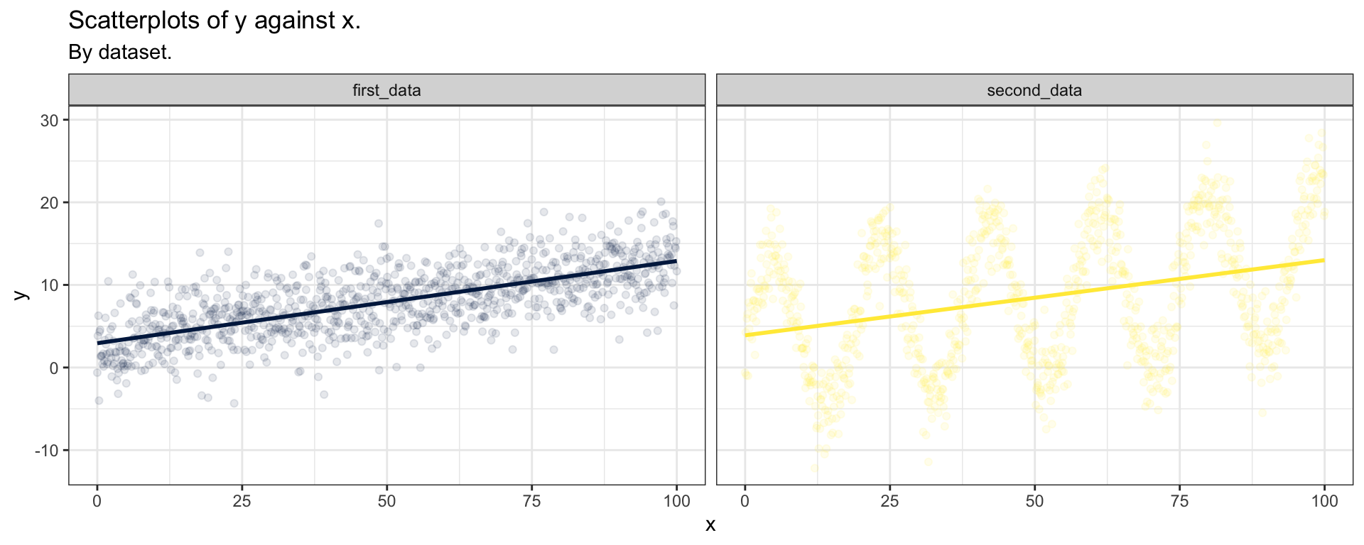
The most important first thing you should do before any modeling attempt is to look at your data.
As you can see, both data sets seem to generate the same linear regression predictions, although we already clearly understand which one will go sideways…
Second step: Modeling
- We know the R function to fit linear regression models is
lm(). - We have seen its syntax for simple models.
- We have been introduced to the broom package for retrieving relevant information from the output of
lm(). - The
broom::glance()help page will provide you with a short summary of the information retrieved byglance(). - The
broom::tidy()help page will provide you with a short summary of the information retrieved bytidy(). - The
broom::augment()help page will provide you with a short summary of the information retrieved byaugment().
Third step: Model Diagnosis
You must always remember that, even though R facilitates computations, it does not verify for you that the assumptions required by the model are met by your data!
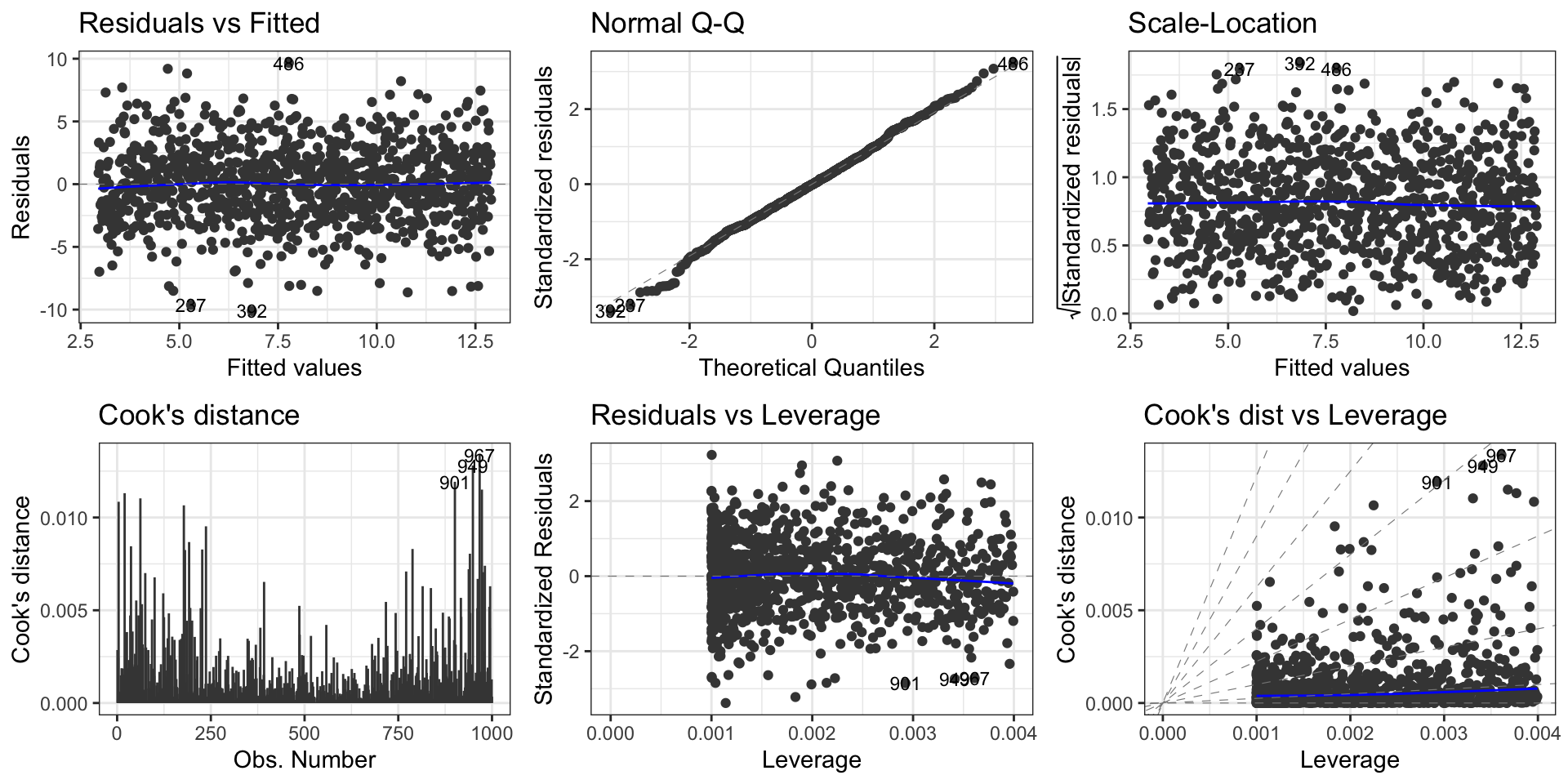
This is where model diagnosis comes into play. You can almost entirely diagnose your model graphically. Using the grammar of graphics in ggplot2, this can be achieved using the ggfortify package.
Reminder: model assumptions (1/3)
Assumptions to check
- Linearity. The relationship between the predictor (x) and the outcome (y) is assumed to be linear.
- Normality. The error terms are assumed to be normally distributed.
- Homogeneity of variance. The error terms are assumed to have a constant variance (homoscedasticity).
- Independence. The error terms are assumed to be independent.
Potential problems to check
Non-linearity of the outcome - predictor relationships
Heteroscedasticity: Non-constant variance of error terms.
Presence of influential and potential outlier values in the data:
- Outliers: typically large standardized residuals
- High-leverage points: typically large leverage values
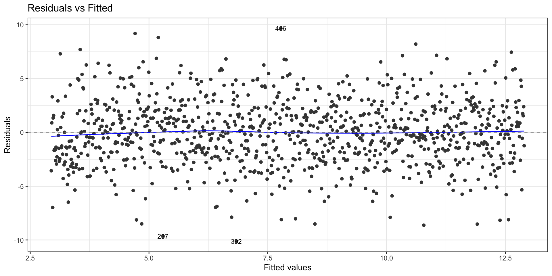
First data set: Residuals vs fitted values
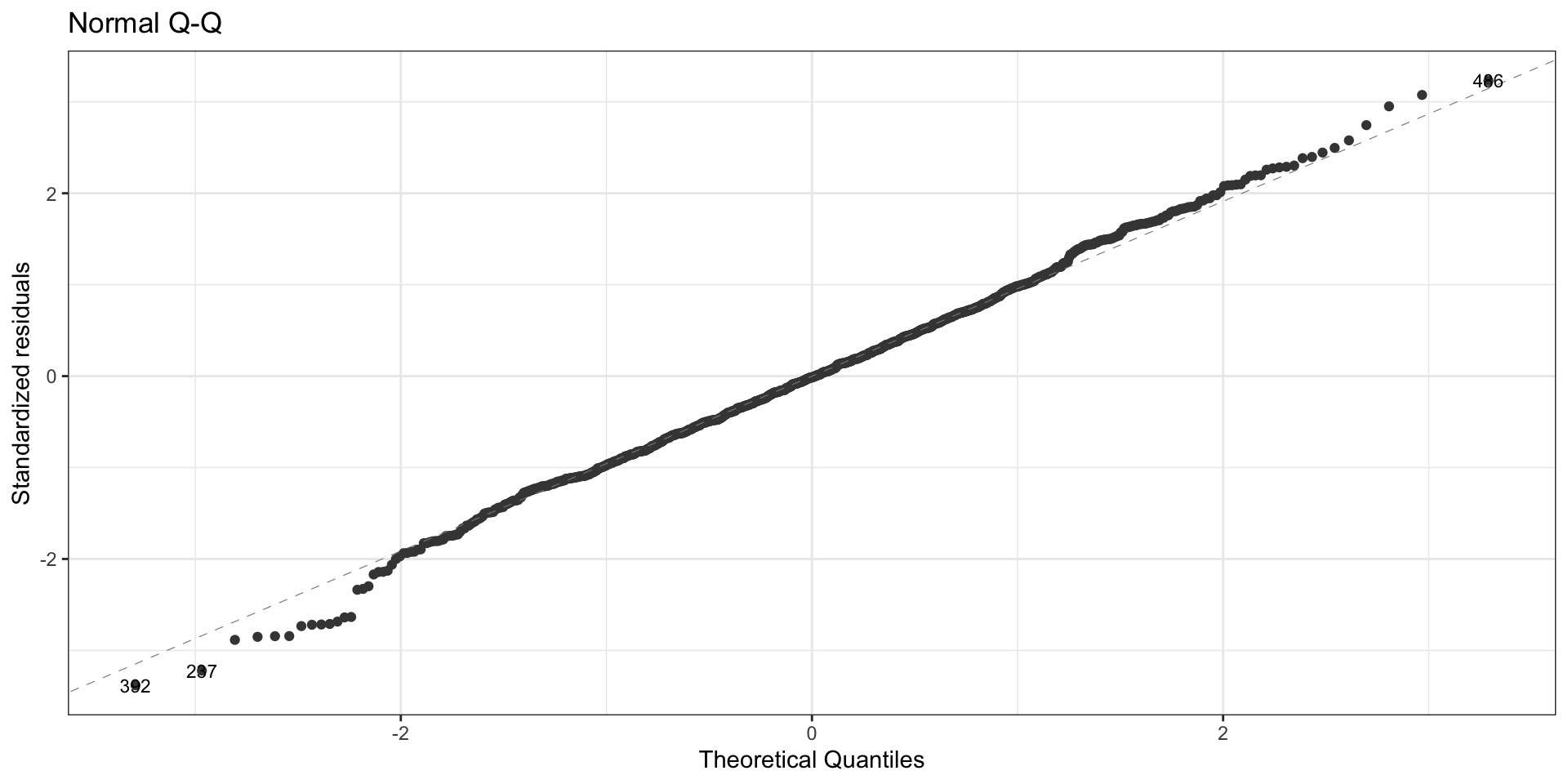
First data set: Normal QQ plot
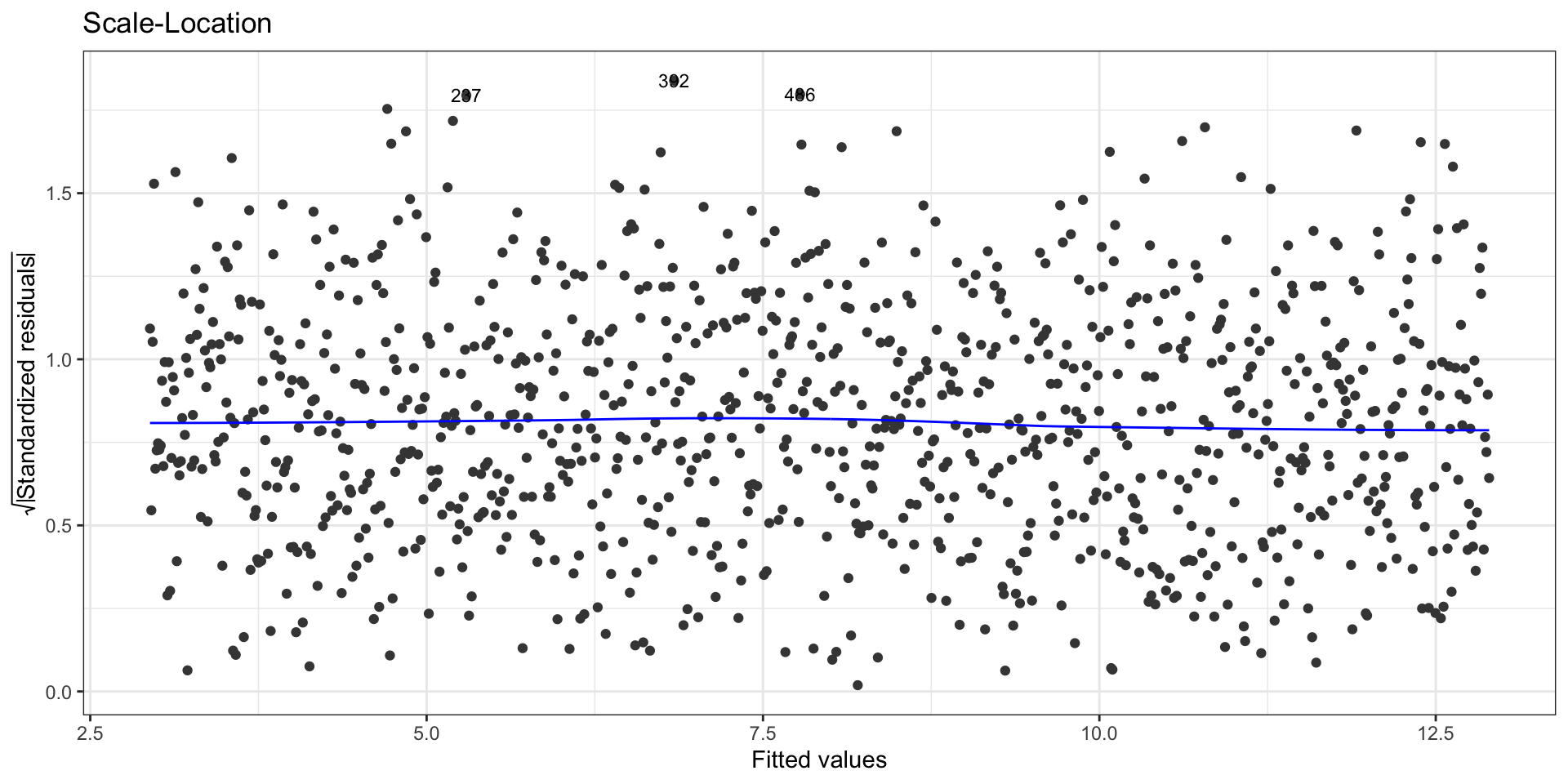
First data set: Scale-location plot
First data set: Influential points, outliers
Usage
To check the zero-mean assumption on the residuals and to spot potential outliers in the top and bottom right corners (residuals vs leverages plot)
To spot potential outliers as observations with the largest Cook’s distance.
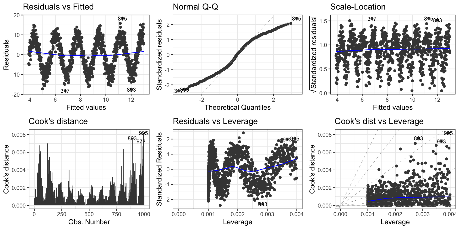
Second data set: Model diagnosis
More complex models
Model specification
The left-hand side of ~ must contain the response variable as named in the atomic vector storing its values or in the data set containing it.
The right-hand side specifies the predictors and will therefore be a combination of potentially transformed variables from your data set (or from atomic vectors defined in your R environment). To get the proper syntax for the rhs of the formula, you should be know the set of allowed operators that have a specific interpretation by R when used within a formula:
+for adding terms.-for removing terms.:for adding interaction terms only.*for crossing variables, i.e. adding variables and their interactions.%in%for nesting variables, i.e. adding one variable and its interaction with another.^for limiting variable crossing to a specified order.for adding all other variables in the matrix that have not yet been included in the model.
Model specification (continued)
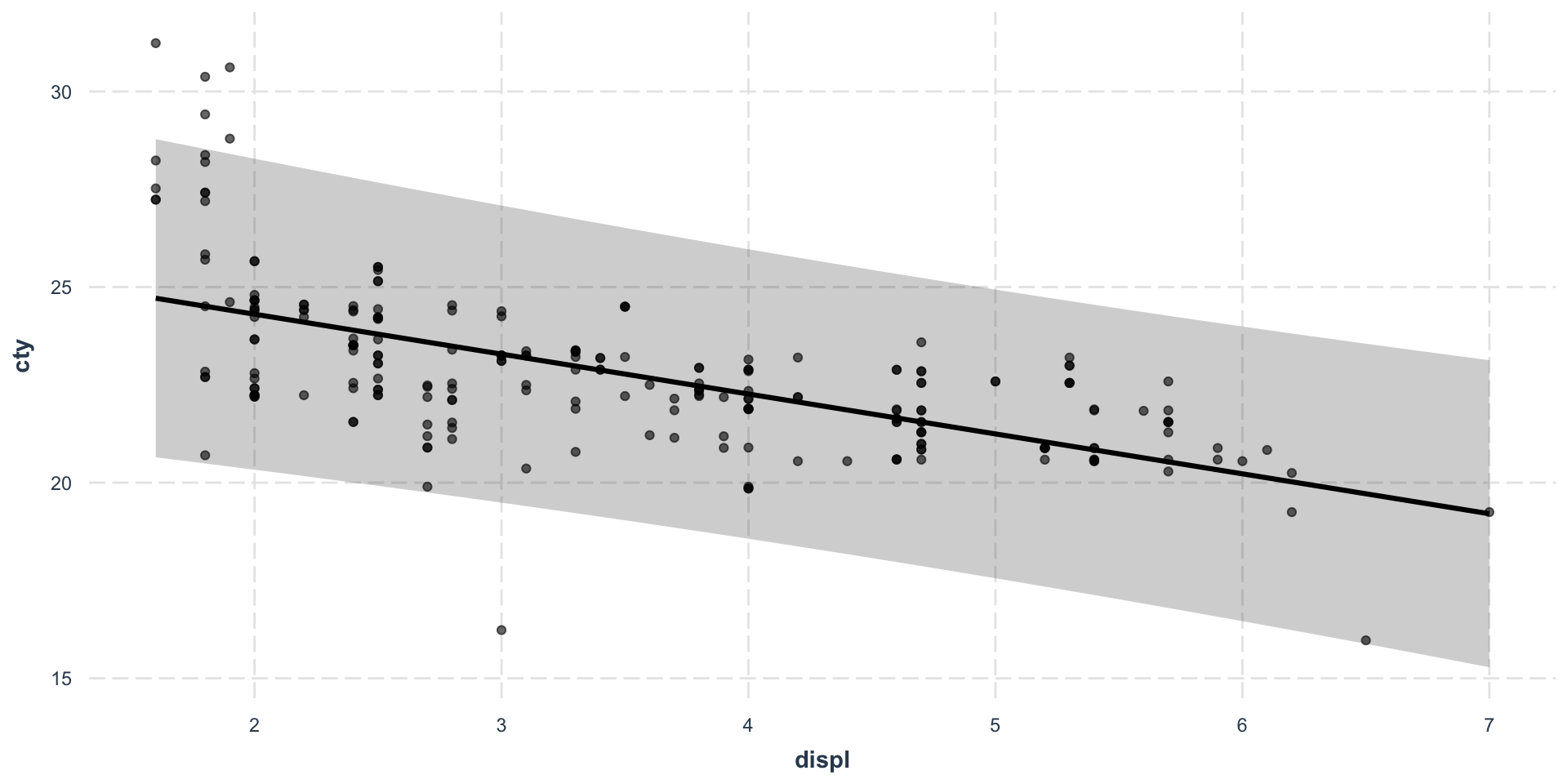
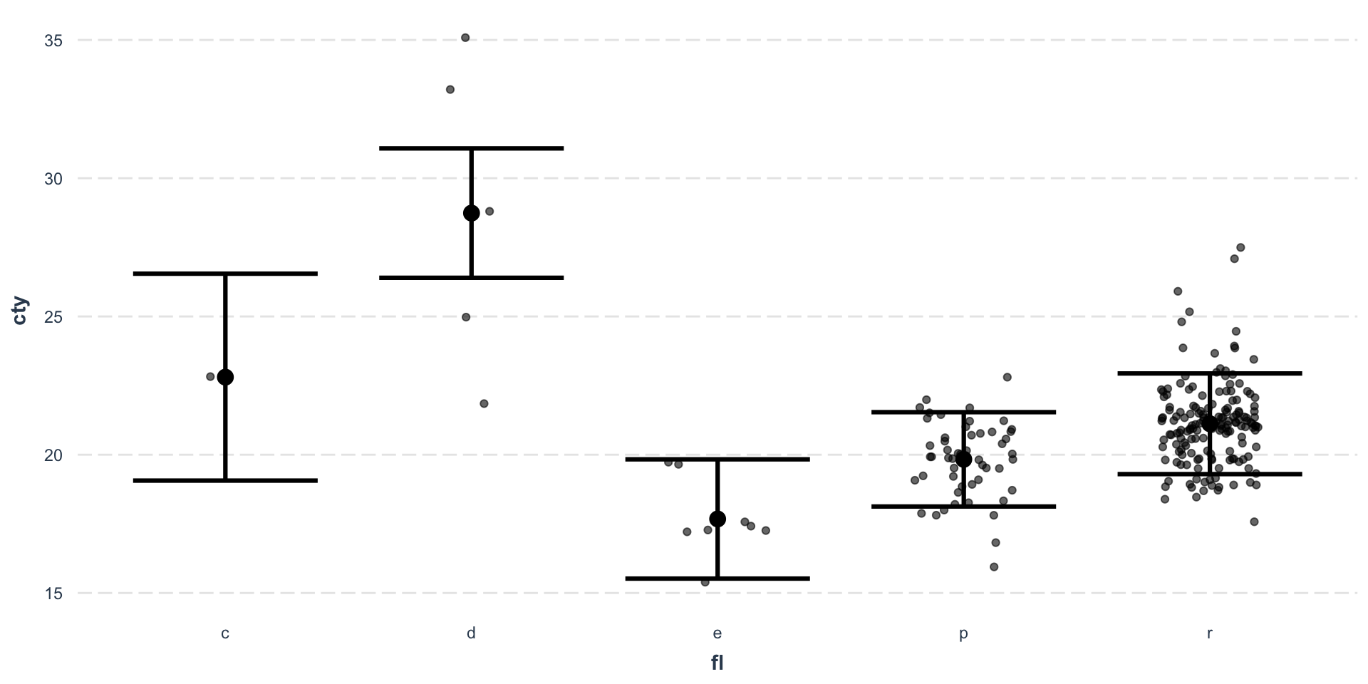
Linear regression assumes that the response variable (y) and at least one predictor (x) are continuous variables. The following table summarizes the effect of operators when adding a variable z to the predictors. When z is categorical, we assume that it can take \(h\) unique possible values \(z_0, z_1, \dots, z_{h-1}\).
Type of z |
Formula | Model |
|---|---|---|
| Continuous | y ~ x + z |
\(Y = \beta_0 + \beta_1 x + \beta_2 z + \varepsilon\) |
| Continuous | y ~ x : z |
\(Y = \beta_0 + \beta_1 x z + \varepsilon\) |
| Continuous | y ~ x * z |
\(Y = \beta_0 + \beta_1 x + \beta_2 z + \beta_3 x z + \varepsilon\) |
| Categorical | y ~ x + z |
\(Y = \beta_0^{(0)} + \sum_{\ell = 1}^{h-1} \beta_\ell^{(0)} \delta_{\{z = z_\ell\}} + \beta_1^{(1)} x + \varepsilon\) |
| Categorical | y ~ x : z |
\(Y = \beta_0^{(0)} + \beta_1^{(1)} x + \sum_{\ell = 1}^{h-1} \beta_\ell^{(1)} x \delta_{\{z = z_\ell\}} + \varepsilon\) |
| Categorical | y ~ x * z |
\(Y = \beta_0^{(0)} + \sum_{\ell = 1}^{h-1} \beta_\ell^{(0)} \delta_{\{z = z_\ell\}} + \beta_0^{(1)} x + \sum_{\ell = 1}^{h-1} \beta_\ell^{(1)} x \delta_{\{z = z_\ell\}} + \varepsilon\) |
I()
What strikes from the previous table is that the natural multiplication of variables within a formula does not simply adds the product of the predictors in the model but also the predictors themselves.
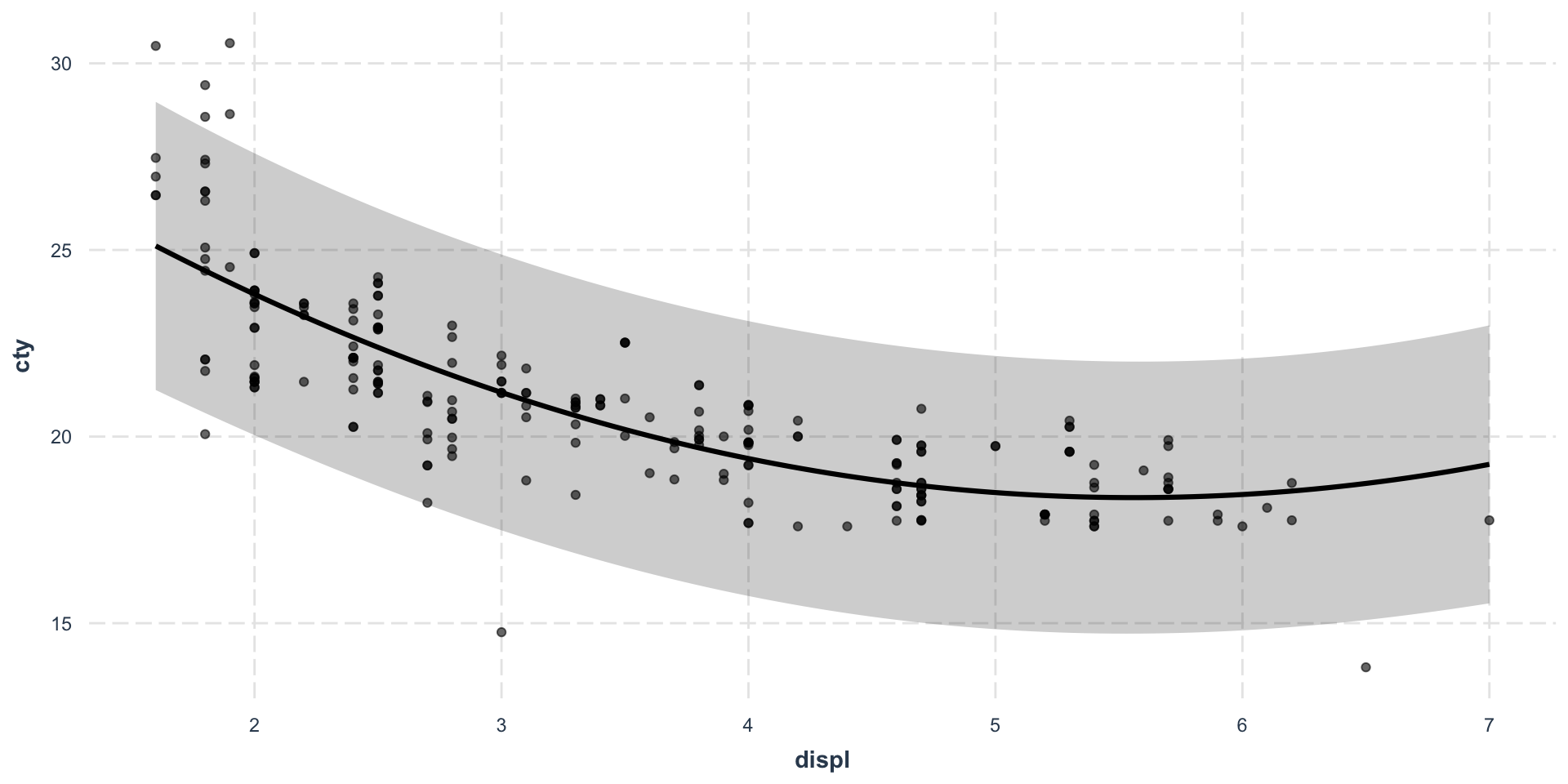
What if you want to actually perform an arithmetic operation on your predictors to include a transformed predictor in your model? For example, you might want to include both \(x\) and \(x^2\) in your model. You have two options:
- You compute all of the (possibly transformed) predictors you want to include in your model beforehand and store them in the data set (remember
dplyr::mutate()which will help you achieve this goal easily); or,- You use the as-is operator
I(). In this case, you instructlm()that the operations declared withinI()must be performed outside from the formula environment and before generating the design matrix for the model.
Effective Model Summaries
There are two possible software suites:
- either
jtoolsandinteractionspackages: - or
ggeffectsandsjPlotpackages.
They both provide tools for summarizing and visualising models, marginal effects, interactions and model predictions.
Tabular summary (1/2)
| Observations | 831 (10 missing obs. deleted) |
| Dependent variable | metascore |
| Type | OLS linear regression |
| F(6,824) | 169.37 |
| R² | 0.55 |
| Adj. R² | 0.55 |
| Est. | S.E. | t val. | p | |
|---|---|---|---|---|
| (Intercept) | -39.96 | 5.92 | -6.75 | 0.00 |
| imdb_rating | 12.80 | 0.49 | 25.89 | 0.00 |
| log(us_gross) | 0.47 | 0.31 | 1.52 | 0.13 |
| genre5Comedy | 6.32 | 1.06 | 5.95 | 0.00 |
| genre5Drama | 7.66 | 1.08 | 7.12 | 0.00 |
| genre5Horror/Thriller | -0.73 | 1.51 | -0.48 | 0.63 |
| genre5Other | 5.86 | 3.25 | 1.80 | 0.07 |
| Standard errors: OLS |
Tabular summary (2/2)
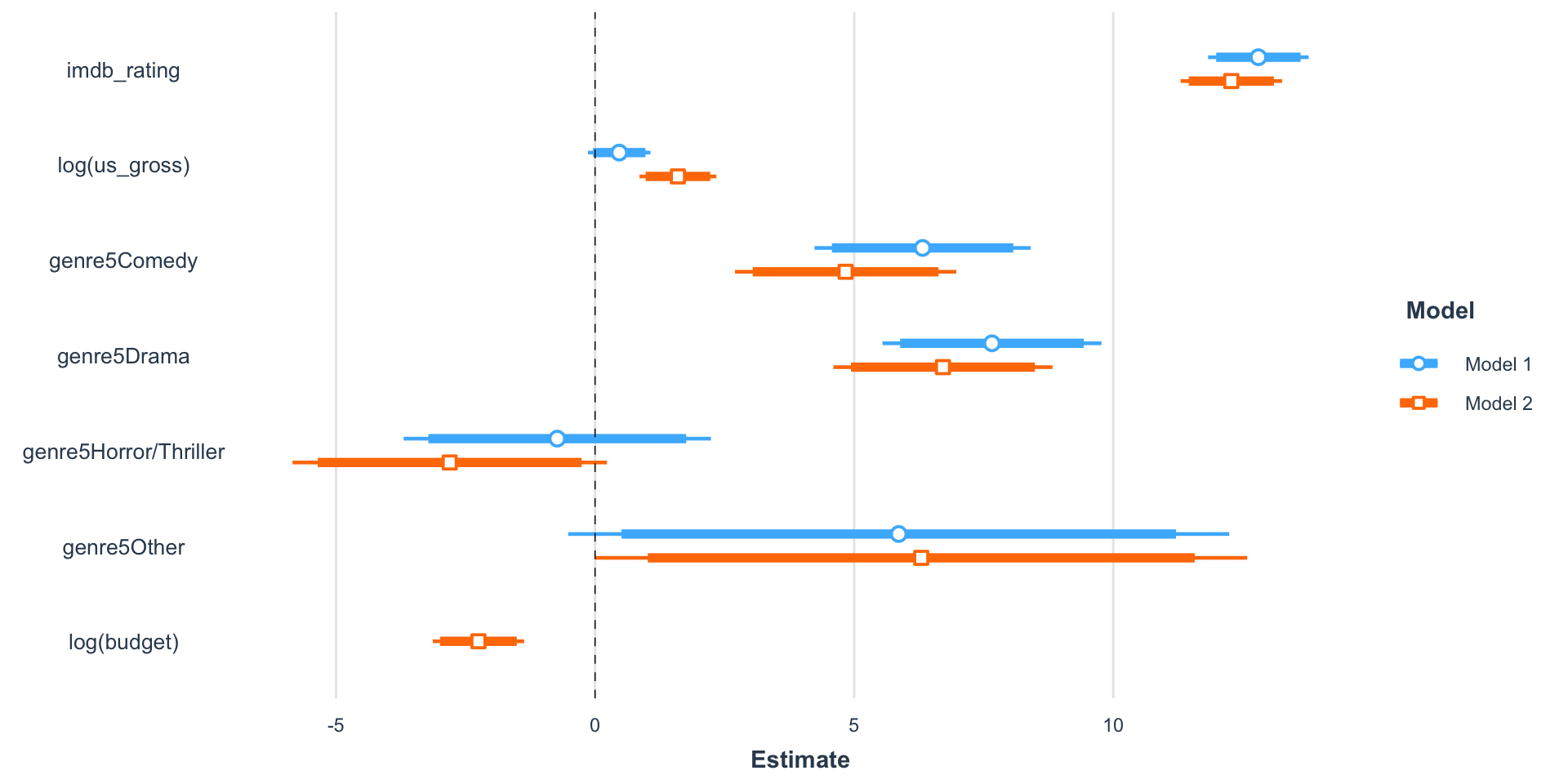
| Model 1 | Model 2 | |||
|---|---|---|---|---|
| (Intercept) | -39.96 *** | [-51.58, -28.34] | -16.47 * | [-31.16, -1.78] |
| imdb_rating | 12.80 *** | [11.83, 13.77] | 12.28 *** | [11.30, 13.26] |
| log(us_gross) | 0.47 | [-0.14, 1.07] | 1.60 *** | [0.86, 2.34] |
| genre5Comedy | 6.32 *** | [4.24, 8.41] | 4.84 *** | [2.70, 6.97] |
| genre5Drama | 7.66 *** | [5.55, 9.77] | 6.71 *** | [4.60, 8.83] |
| genre5Horror/Thriller | -0.73 | [-3.70, 2.24] | -2.81 | [-5.84, 0.23] |
| genre5Other | 5.86 | [-0.52, 12.24] | 6.30 * | [0.01, 12.59] |
| log(budget) | -2.25 *** | [-3.13, -1.37] | ||
| N | 831 | 831 | ||
| R2 | 0.55 | 0.57 | ||
| *** p < 0.001; ** p < 0.01; * p < 0.05. | ||||
Visual summary
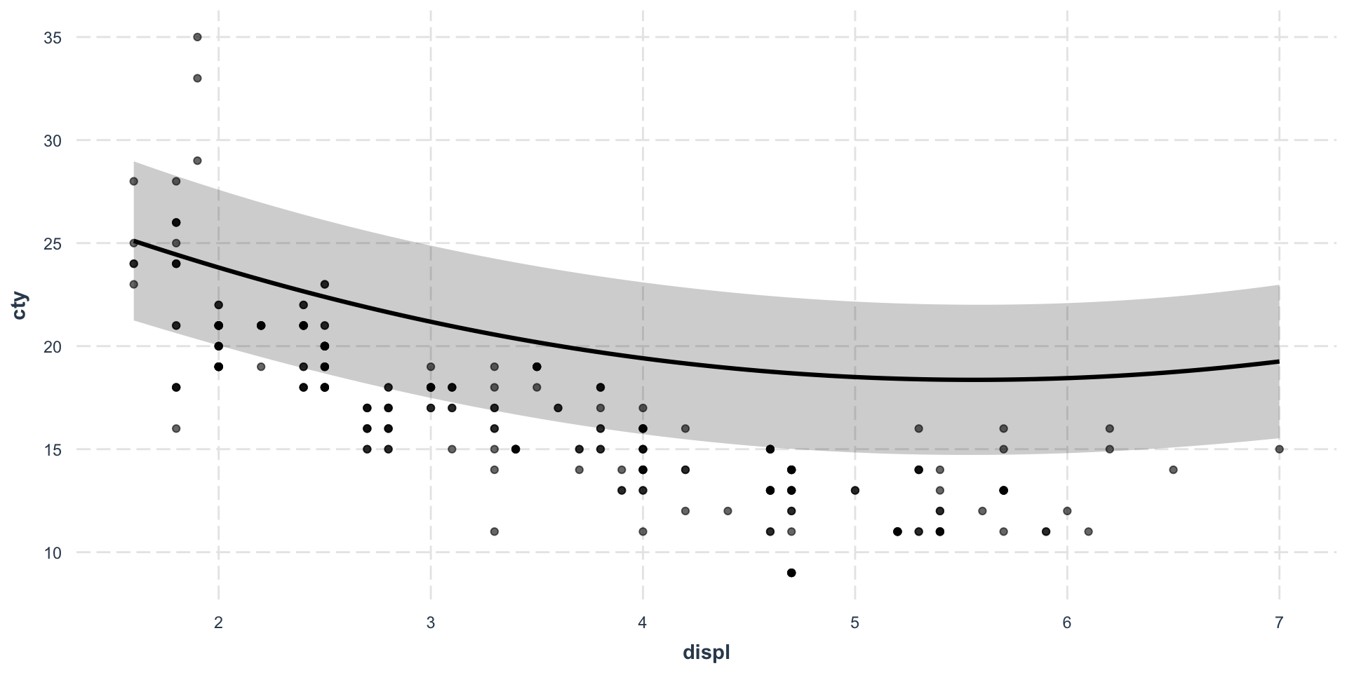
Effect plot - Continuous predictor
Effect plot - Categorical predictor
Interaction plots
This is handled by the interaction package.
Johnson-Neyman plot:
sim_slopes()Two-way interaction with at least one continuous predictor:
interact_plot()Two-way interaction between categorical predictors:
cat_plot()
Collinearity & Multicollinearity
(Multi)-collinearity refers to high correlation in two or more independent variables in the regression model.
Multicollinearity can arise from poorly designed experiments (Data-based multicollinearity) or from creating new independent variables related to the existing ones (structural multicollinearity).
Correlation plots are a great tool to explore colinearity between two variables. They can be seamlessly computed and visualized using packages such as
corrrorggcorrplot.
Variation Inflation Factor (1/3)
The Variance inflation factor (VIF) measures the degree of multicollinearity or collinearity in the regression model.
\[ \mathrm{VIF}_i = \frac{1}{1 - R_i^2}, \]
where \(R_i^2\) is the multiple correlation coefficient associated to the regression of \(X_i\) against all remaining independent variables.
Variation Inflation Factor (2/3)
You can add VIFs to the summary of a model as follows:
| Observations | 234 |
| Dependent variable | cty |
| Type | OLS linear regression |
| F(13,220) | 100.37 |
| R² | 0.86 |
| Adj. R² | 0.85 |
| Est. | S.E. | t val. | p | VIF | |
|---|---|---|---|---|---|
| (Intercept) | -199.79 | 51.14 | -3.91 | 0.00 | NA |
| displ | -1.02 | 0.29 | -3.53 | 0.00 | 11.76 |
| year | 0.12 | 0.03 | 4.52 | 0.00 | 1.11 |
| cyl | -0.85 | 0.20 | -4.26 | 0.00 | 8.69 |
| classcompact | -2.81 | 1.00 | -2.83 | 0.01 | 3.69 |
| classmidsize | -2.95 | 0.97 | -3.05 | 0.00 | 3.69 |
| classminivan | -5.08 | 1.05 | -4.82 | 0.00 | 3.69 |
| classpickup | -5.89 | 0.92 | -6.37 | 0.00 | 3.69 |
| classsubcompact | -2.63 | 1.01 | -2.61 | 0.01 | 3.69 |
| classsuv | -5.59 | 0.88 | -6.33 | 0.00 | 3.69 |
| fld | 5.93 | 1.85 | 3.21 | 0.00 | 1.60 |
| fle | -5.13 | 1.81 | -2.84 | 0.00 | 1.60 |
| flp | -2.97 | 1.72 | -1.73 | 0.08 | 1.60 |
| flr | -1.69 | 1.70 | -0.99 | 0.32 | 1.60 |
| Standard errors: OLS |
Variation Inflation Factor (3/3)
- VIFs are always at least equal to 1.
- In some domains, VIF over 2 is worthy of suspicion. Others set the bar higher, at 5 or 10. Others still will say you shouldn’t pay attention to these at all.
- Small effects are more likely to be drowned out by higher VIFs, but this may just be a natural, unavoidable fact with your model (e.g., there is no problem with high VIFs when you have an interaction effect).
Model selection
Forward selection
- Start with no variables in the model.
- Test the addition of each variable using a chosen model fit criterion1, adding the variable (if any) whose inclusion gives the most statistically significant improvement of the fit
- Repeat until none improves the model to a statistically significant extent.
Backward elimination
- Start with all candidate variables
- Test the deletion of each variable using a chosen model fit criterion, deleting the variable (if any) whose loss gives the most statistically insignificant deterioration of the model fit
- Repeat until no further variables can be deleted without a statistically significant loss of fit.

Data Science with R - aymeric.stamm@cnrs.fr - https://astamm.github.io/data-science-with-r/
