Dimensionality reduction

If you’ve worked with a lot of variables before, you know this can present problems. Do you understand the relationships between each variable? Do you have so many variables that you are in danger of overfitting your model to your data or that you might be violating assumptions of whichever modeling tactic you’re using?

You might ask the question, “How do I take all of the variables I’ve collected and focus on only a few of them?” In technical terms, you want to “reduce the dimension of your feature space.” By reducing the dimension of your feature space, you have fewer relationships between variables to consider and you are less likely to overfit your model.

Think about linear regression:

multicollinearity issues;
difficult to use strategies like backward elimination.

PCA

What ?

Principal component analysis is a technique for feature extraction — so it combines our input variables in a specific way, then we can drop the “least important” variables while still retaining the most valuable parts of all of the variables! As an added benefit, each of the “new” variables after PCA are all independent of one another.

How ?

The dimension reduction is achieved by identifying the principal directions, called principal components, in which the data varies.

PCA assumes that the directions with the largest variances are the most “important” (i.e, the most principal).

When to use?

Do you want to reduce the number of variables, but aren’t able to identify variables to completely remove from consideration?
Do you want to ensure your variables are independent of one another?
Are you comfortable making your independent variables less interpretable?

Principle

The 1st principal component (PC) accounts for the largest possible variance in the data set;
i.e. the line in which the projection of the points (red dots) is the most spread out.
The second PC is uncorrelated to the 1st PC and maximizes the remaining variance;
etc.

Mathematical formalism

Context.

X₁, …, X_n a sample of n i.i.d. random vectors in ℝ^p. Let 𝕏 = (X₁, …, X_n)^⊤ be the n × p data matrix, whose j-th column is the vector x_j containing the n observations on the j-th variable. Let Σ be the covariance structure of the X_i’s.

Determination of the 1st PC

The 1st principal component (PC) accounts for the largest possible variance in the data set.

Search a linear projection a ∈ ℝ^p of the original variables (columns of 𝕏) with maximal variance. Such projection reads 𝕏a of which each component has variance: Var([𝕏a]_i) = a^⊤Σa.

Requires additional constraint because maximum does not exist in ℝ^p: search for ∥a∥ = 1.
The sample covariance S is an unbiased estimator of Σ, hence we can instead solve: $$ \max_{\mathbf{a} \in \mathcal{S}^{p-1}} \mathbf{a}^\top S \mathbf{a} = \max_{\mathbf{a} \in \mathbb{R}^p} \frac{\mathbf{a}^\top S \mathbf{a}}{\mathbf{a}^\top \mathbf{a}} $$
Solution is eigenvector of S associated to the largest eigenvalue:
- constrained problem is equivalent to maximizing a^⊤Sa − λ(a^⊤a − 1);
- differentiation leads to Sa = λa; hence, a is an eigenvector of S;
- hence we get a^⊤Sa = λ which means that λ must be the largest eigenvalue of S in order to maximize a^⊤Sa.

R Packages

Principal Component Computation

prcomp() and princomp() from built-in R stats package,
PCA() from FactoMineR package,
dudi.pca() from ade4 package.

Recommendation

The FactoMineR::PCA() function.

Information Extraction and Visualization

The factoextra package.

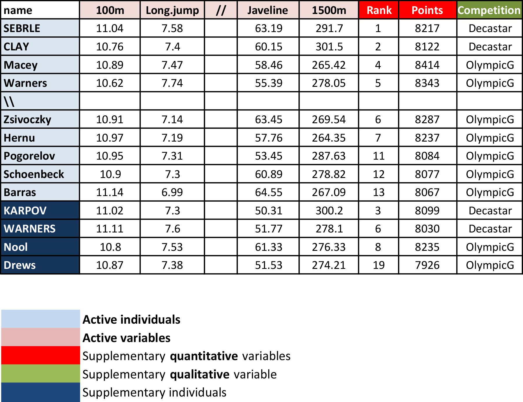
Case Study

Athletes’ performance during two sporting events (Decastar and OlympicG)
It contains 41 individuals (athletes) described by 13 variables.

Objectives

PCA allows to describe a data set, to summarize a data set, to reduce the dimensionality. We want to perform a PCA on all the individuals of the data set to answer several questions:

Individuals’ study (athletes’ study)

Two athletes will be close to each other if their results to the events are close. We want to see the variability between the individuals.

Are there similarities between individuals for all the variables?
Can we establish different profiles of individuals?
Can we oppose a group of individuals to another one?

Variables’ study (performances’ study)

We want to see if there are linear relationships between variables. The two objectives are to summarize the correlation matrix and to look for synthetic variables: can we resume the performance of an athlete by a small number of variables?

Link between this two studies

Can we characterize groups of individuals by variables?

PCA Terminology

Active individuals: Individuals used for PCA.

Supplementary individuals: Coordinates of these individuals will be predicted using the PCA information and parameters obtained using active individuals.

Active variables: Variables used for PCA.

Supplementary variables: Coordinates of these variables will be predicted also. These can be:

Supplementary continuous variables: Cols 11 and 12 correspond respectively to the rank and the points of athletes.
Supplementary qualitative variables: Col 13 corresponds to the two athletic meetings (2004 Olympic Game or 2004 Decastar). This is a categorical variable. It can be used to color individuals by groups.

Data standardization

Description of the problem

PCA linearly combines original variables to maximize variance
If one variable is measured in meter and another in centimeter, the first one will contribute more to the variance than the second one, even if the intrinsic variability of each variable is the same.

⇒ We need to scale the variables prior to performing PCA!

A common solution: Standardization

$$ x_{ij} \leftarrow \frac{x_{ij} - \overline{x}_j}{\sqrt{\frac{1}{n-1} \sum_{\ell=1}^n (x_{\ell j} - \overline{x}_j)^2}} $$

⇒ The function PCA() in FactoMineR, standardizes the data automatically.

`PCA()` Syntax

PCA(
  # a data frame with n rows (individuals) and p columns (numeric variables)
  X = , 
  
  # number of dimensions kept in the results (by default 5)
  ncp = , 
  
  # a vector indicating the indexes of the supplementary individuals
  ind.sup = , 
  
  # a vector indicating the indexes of the quantitative supplementary variables
  quanti.sup = ,
  
  # a vector indicating the indexes of the categorical supplementary variables
  quali.sup = , 
  
  # boolean, if TRUE (default) a graph is displayed
  graph = 
)

Running `PCA()`

PCA(X = decathlon[, 1:10], graph = FALSE)

**Results for the Principal Component Analysis (PCA)**
The analysis was performed on 41 individuals, described by 10 variables
*The results are available in the following objects:

   name               description                          
1  "$eig"             "eigenvalues"                        
2  "$var"             "results for the variables"          
3  "$var$coord"       "coord. for the variables"           
4  "$var$cor"         "correlations variables - dimensions"
5  "$var$cos2"        "cos2 for the variables"             
6  "$var$contrib"     "contributions of the variables"     
7  "$ind"             "results for the individuals"        
8  "$ind$coord"       "coord. for the individuals"         
9  "$ind$cos2"        "cos2 for the individuals"           
10 "$ind$contrib"     "contributions of the individuals"   
11 "$call"            "summary statistics"                 
12 "$call$centre"     "mean of the variables"              
13 "$call$ecart.type" "standard error of the variables"    
14 "$call$row.w"      "weights for the individuals"        
15 "$call$col.w"      "weights for the variables"

Visualization and Interpretation

The factoextra package

It helps with interpretation of PCA.
No matter what function you decide to use (stats::prcomp(), FactoMiner::PCA(), ade4::dudi.pca(), ExPosition::epPCA()), you can easily extract and visualize the results of PCA using R functions provided in the factoextra R package.

Useful extraction and visualization functions

get_eigenvalue(): Extract the eigenvalues/variances of principal components.
fviz_screeplot(): Visualize the eigenvalues / proportion of explained variance.
get_pca_ind(), get_pca_var(): Extract the results for individuals and variables, respectively.
fviz_pca_ind(), fviz_pca_var(): Visualize the results individuals and variables, respectively.
fviz_pca_biplot(): Make a biplot of individuals and variables.

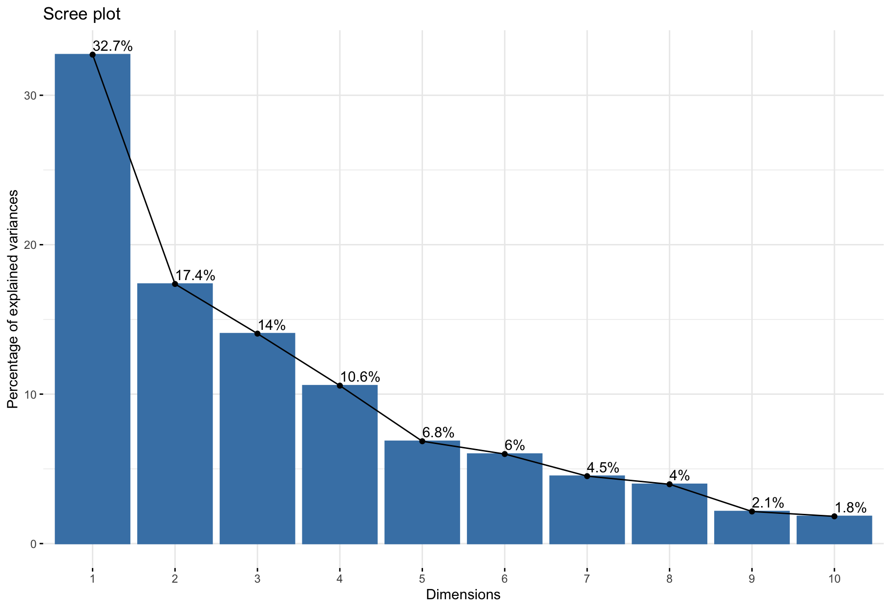
Choice of the reduced dimension

Eigenvalues / Variances

Eigenvalues measure the amount of variation retained by each principal component.

eig_val <- get_eigenvalue(res_pca)
html_table(eig_val)

Choosing the appropriate number of PCs

Eigenvalues can be used to determine the number of principal components to retain after PCA.

Guidelines.

An eigenvalue > 1 indicates that PCs account for more variance than accounted by one of the original variables in standardized data. This is commonly used as a cutoff point for which PCs are retained. This holds true only when the data are standardized.
Balance between a small number to achieve dimensionality reduction well and proporition of total variance explained.
Look at the first few principal components to find interesting patterns in the data.

Graphical tool.

fviz_screeplot(res_pca, addlabels = TRUE)

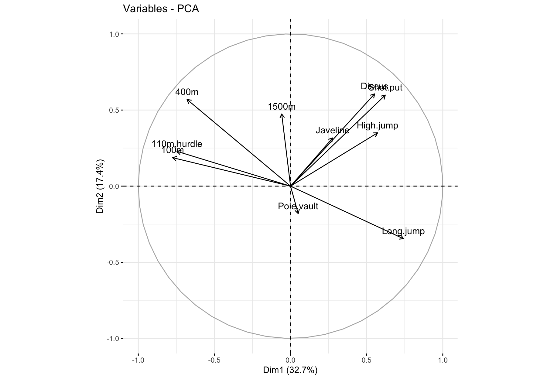
Analysis of the variables

Variable Information in PCA

Variable information extraction

var_info <- get_pca_var(res_pca)

Components

var_info$coord: Coordinates for the variables.
var_info$cos2: Quality of representation of variables by PC: var.cos2 = var.coord * var.coord.
var_info$contrib: Contributions of the variables to the principal components: (var.cos2 * 100) / (sum cos2 of the component).

Usage

Investigate the ability of PCs to strongly represent variables.
Describe each PC in terms of the most contributing variables.

`$coord`: Correlation variables & components

Property: norms of column vectors is 1 (eigenvectors).
Consequence: each coordinate is in [-1,1].

Contribution of PCs to variables

`fviz_pca_var()`: Correlation circle

fviz_pca_var(res_pca, col.var = "black")

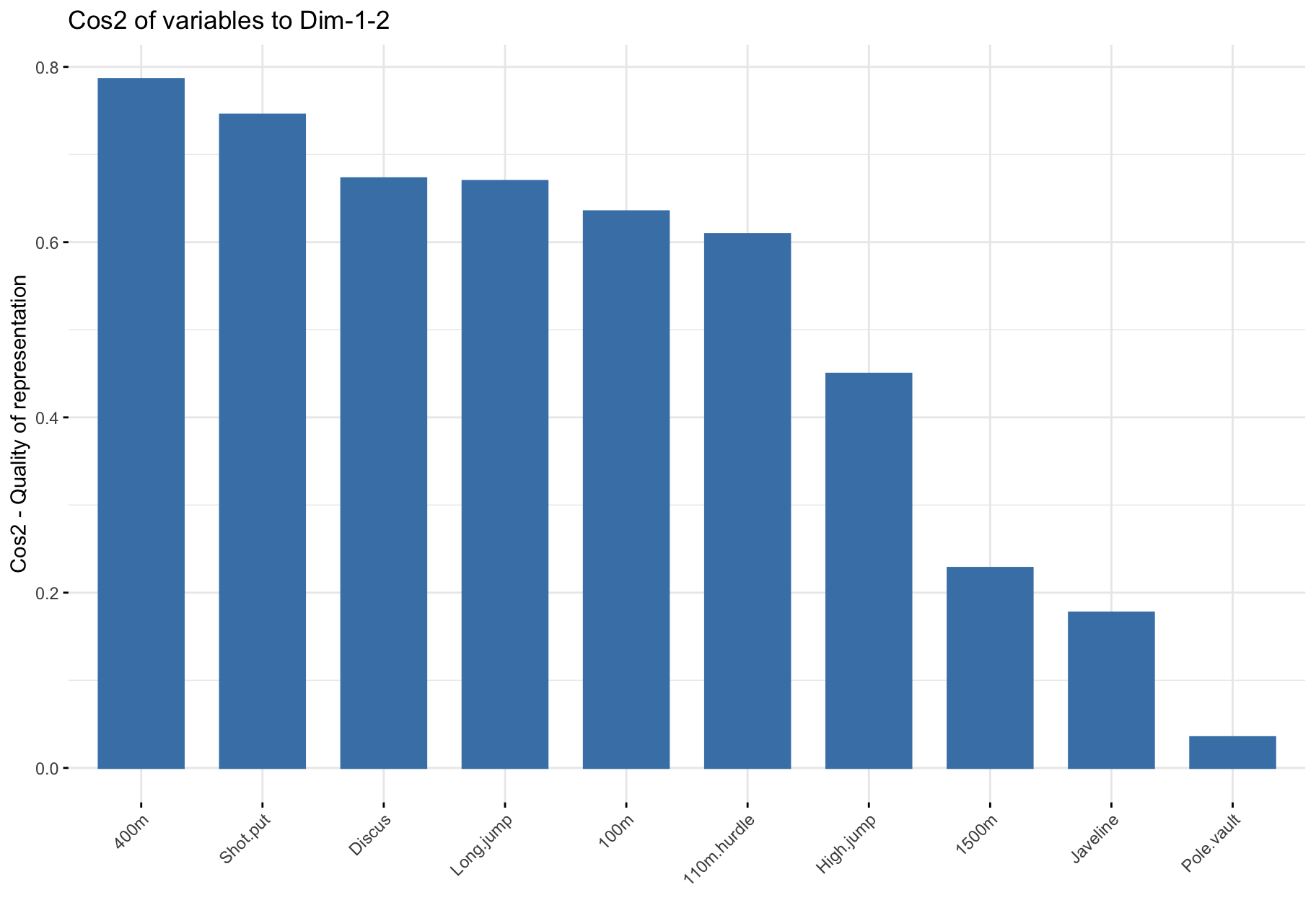
`$cos2`: Quality of representation

Positive and negative strong correlations of PCs to a given variable imply that the PCs represent it well.
Squared correlations thus measure quality of representation.

`$cos2`: Graphical tool 1

corrplot::corrplot(var_info$cos2, is.corr = FALSE)

`$cos2`: Graphical tool 2

# Total cos2 of variables on Dim.1 and Dim.2
factoextra::fviz_cos2(res_pca, choice = "var", axes = 1:2)

`$cos2`: Summary

The cos2 values are used to estimate the quality of the representation.
High cos2 indicates a good representation of the variable by the corresponding PC.
Low cos2 indicates that the variable is poorly represented by the corresponding PC.
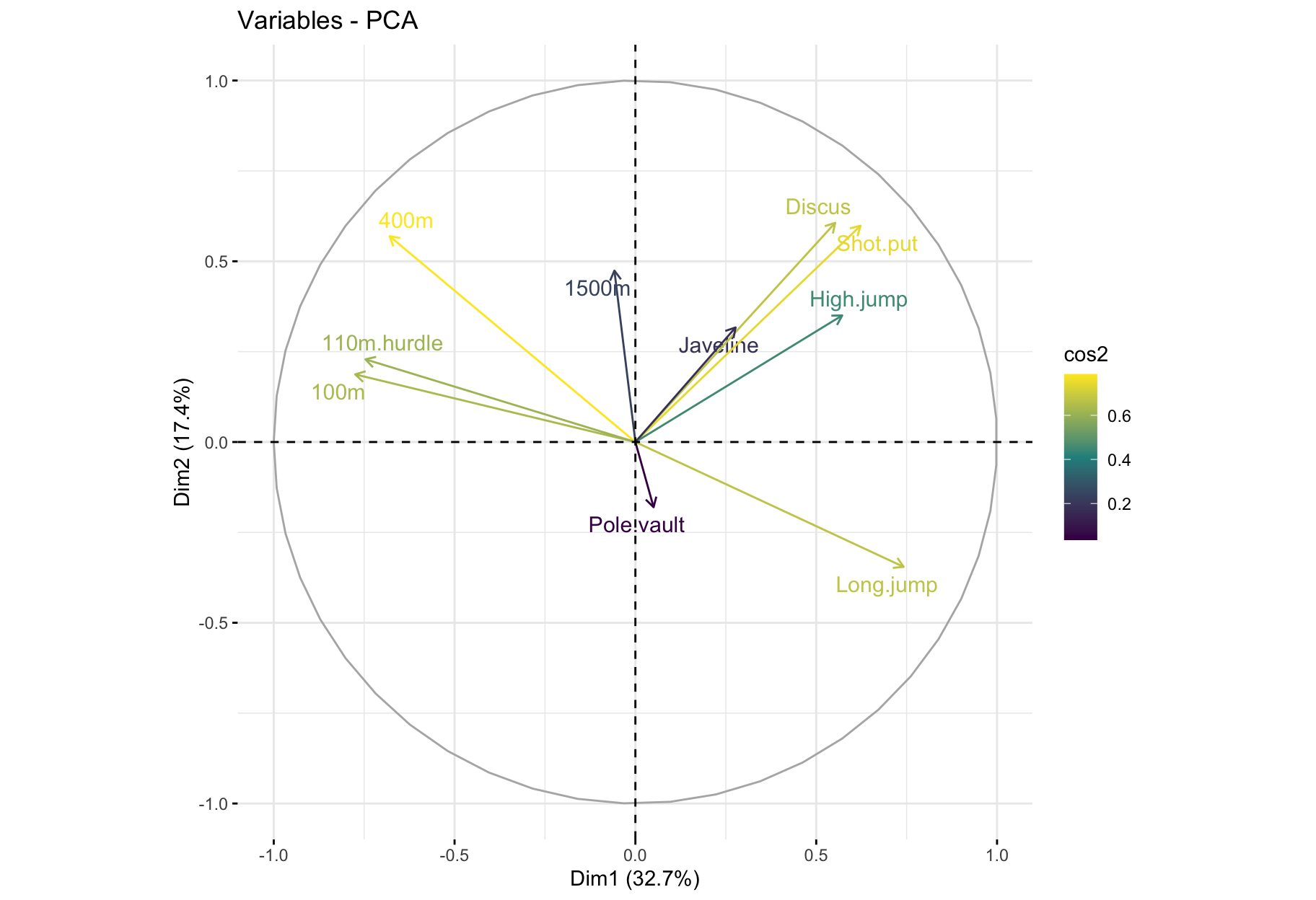
Variables close to circle in plot are very well represented by the 1st two PCs.
Variables close to center in plot are not well represented by the 1st two PCs.

factoextra::fviz_pca_var(X = res_pca, 
                         col.var = "cos2",
                         gradient.cols = viridis::viridis(3),
                         repel = TRUE) # Avoid text overlapping

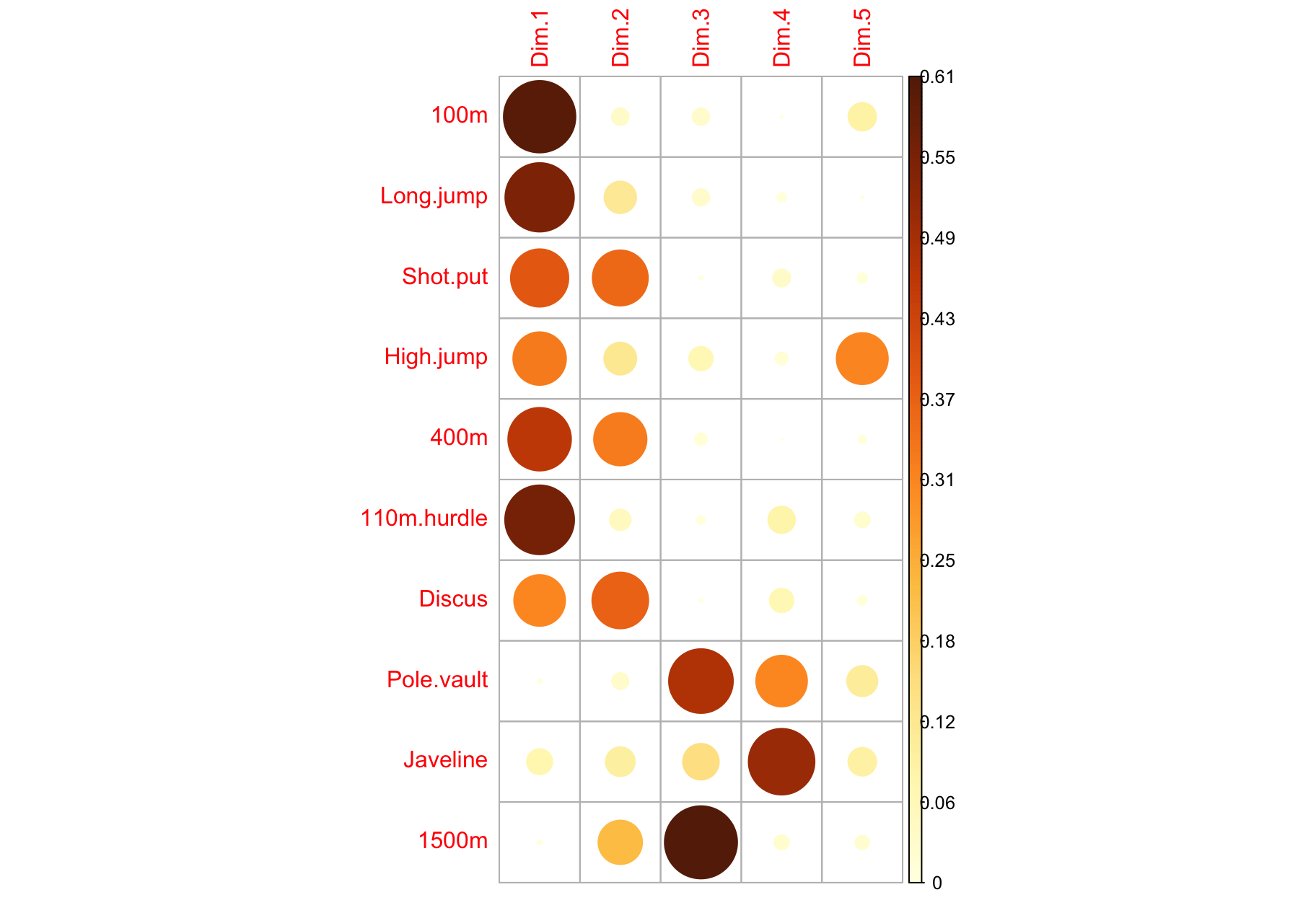
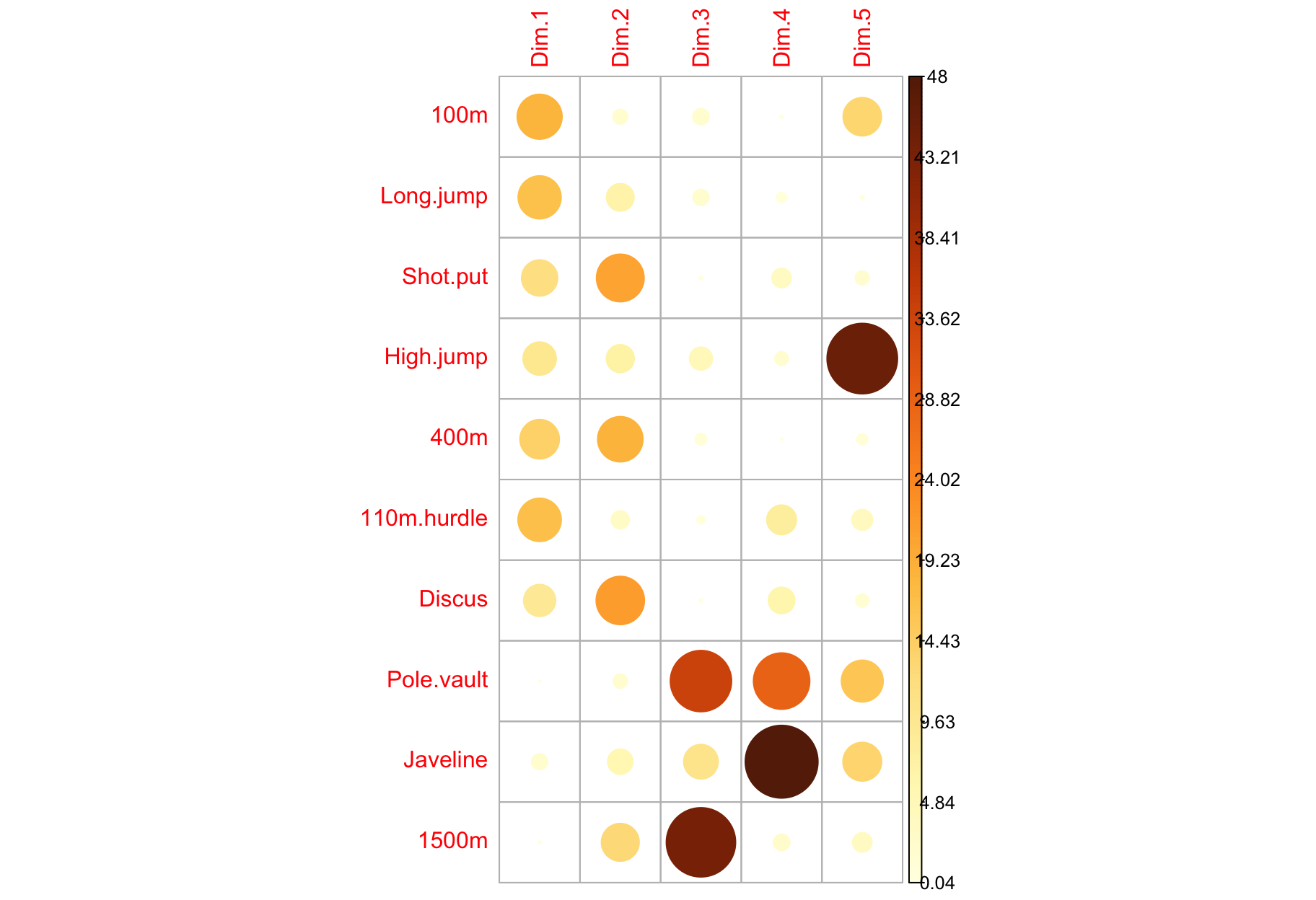
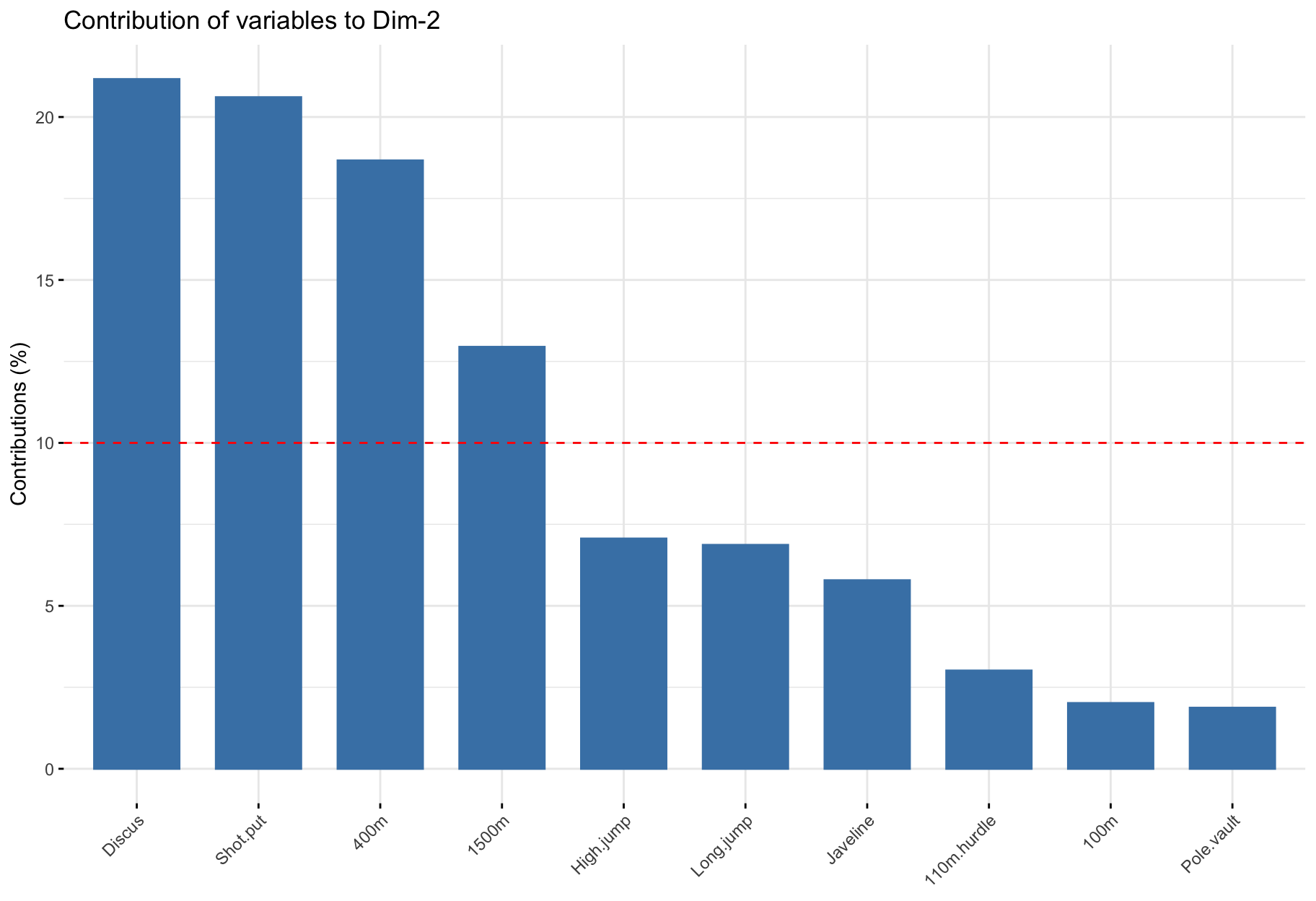
Contribution of variables to PCs

`$contrib`: Important variables

Variables correlating with Dim.1 (PC1) and Dim.2 (PC2) are the most important to explain the variability in the data set.
Variables that do not correlate with any PC or only with the last ones are variables might be removed to simplify the overall analysis.

`$contrib`: Graphical tool 1

corrplot::corrplot(var_info$contrib, is.corr = FALSE)

`$contrib`: Graphical tool 2

# Contributions of variables to PC1
factoextra::fviz_contrib(
  X = res_pca, 
  choice = "var", 
  axes = 1, 
  top = 10
)

# Contributions of variables to PC2
factoextra::fviz_contrib(
  X = res_pca, 
  choice = "var", 
  axes = 2, 
  top = 10
)

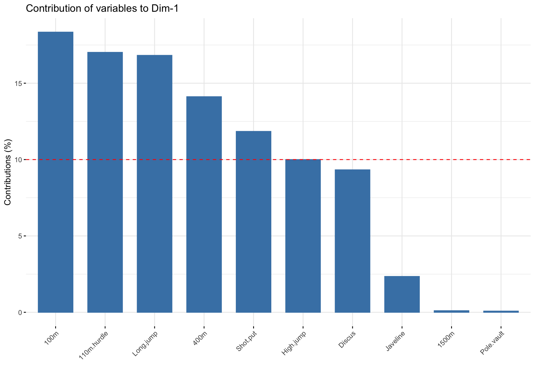
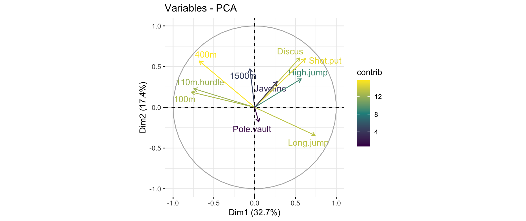
`$contrib`: Summary

factoextra::fviz_pca_var(
  X = res_pca, 
  col.var = "contrib",
  gradient.cols = viridis::viridis(3),
  repel = TRUE
)

Component description

res_pca_var_desc <- FactoMineR::dimdesc(res = res_pca, axes = c(1, 2), proba = 0.05)

Description of PC1

Description of PC2

Analysis of the individuals

The reduced space

Individual information extraction

ind_info <- get_pca_ind(res_pca)

Components

ind_info$coord: Coordinates of the individuals.
ind_info$cos2: Quality of representation of individuals by PC: ind.cos2 = ind.coord * ind.coord.
ind_info$contrib: Contributions of the individuals to the principal components: (ind.cos2 * 100) / (sum cos2 of the component).

Usage

The reduced space should allow easier identification of patterns, provided that it represents them well.
Individuals that are similar are grouped together on the plot.

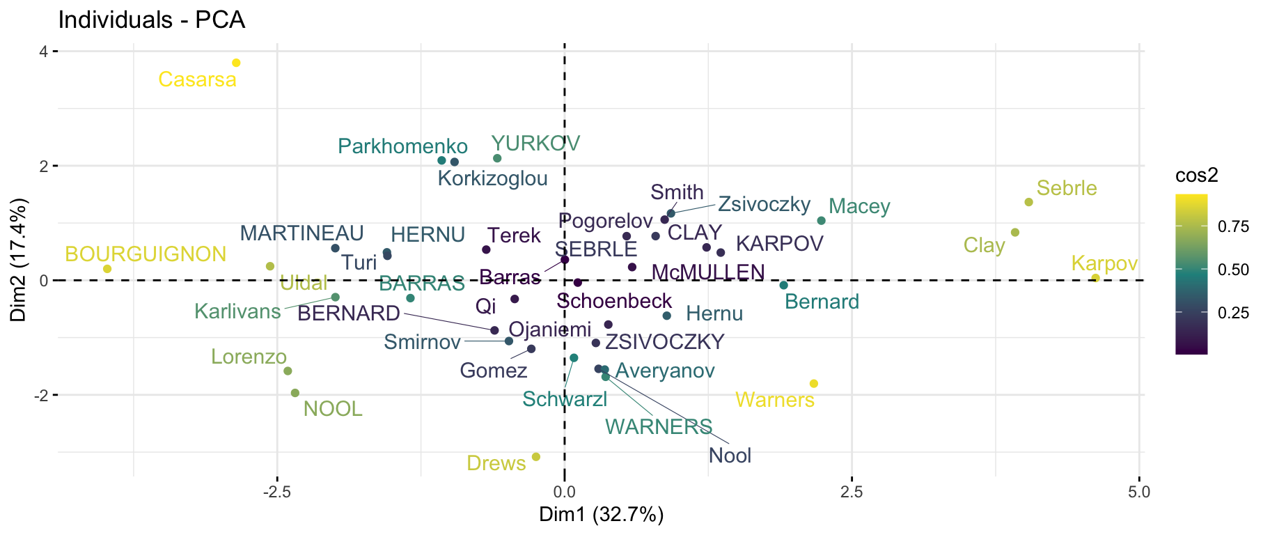
First factorial plane & quality

factoextra::fviz_pca_ind(
  X = res_pca, 
  col.ind = "cos2", 
  gradient.cols = viridis::viridis(3),
  repel = TRUE # Avoid text overlapping (slow if many points)
)

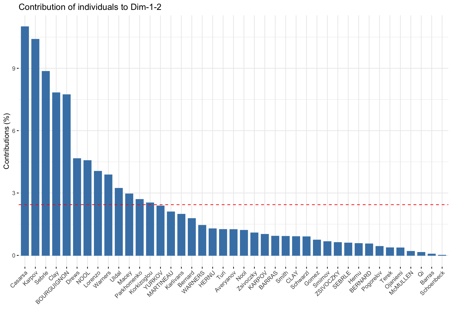
First factorial plane & contribution

# Total contribution on PC1 and PC2
factoextra::fviz_contrib(res_pca, choice = "ind", axes = 1:2)

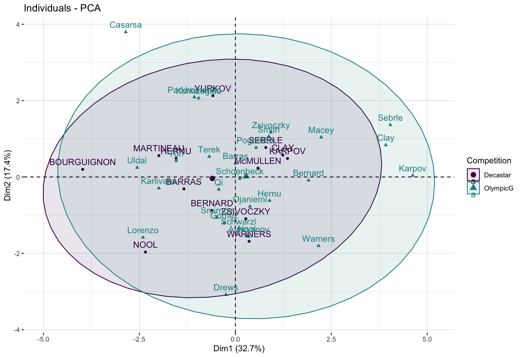
First factorial plane colored by groups

factoextra::fviz_pca_ind(
  X = res_pca,
  col.ind = decathlon$competition[1:23], # color by groups
  palette = viridis::viridis(3),
  addEllipses = TRUE, # Concentration ellipses
  legend.title = "Competition"
)

This plot is useful to understand the ability of a factorial plane to discriminate individuals based on some feature.
Here, we see a tendency with positive score on PC1 for athletes at the Olympics and negative PC1 scores for athletes at the Decastar.
But, ellipses seem to overlap significantly.

Combined variable and individual analysis

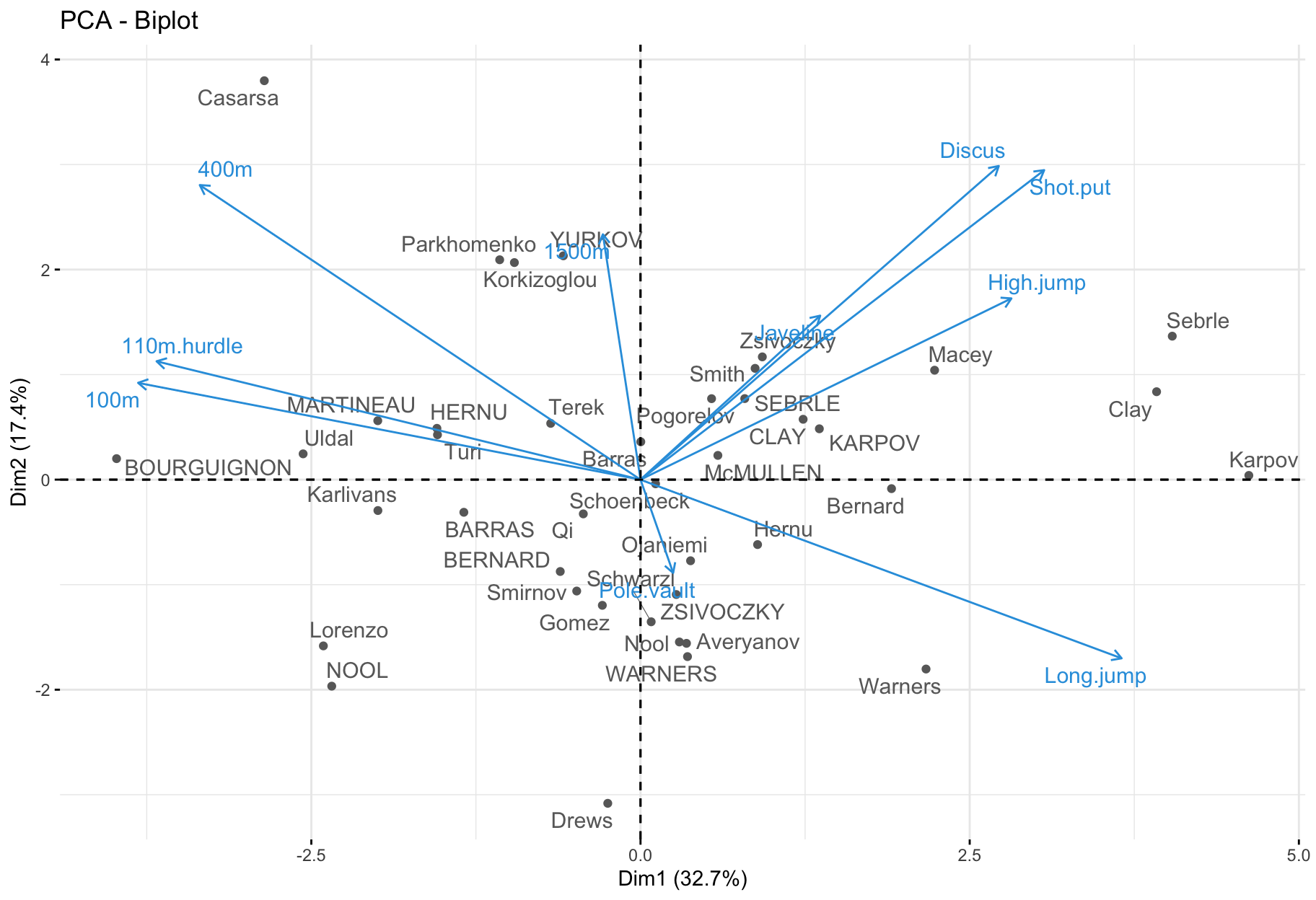
Biplot

factoextra::fviz_pca_biplot(
  X = res.pca, 
  repel = TRUE,
  col.var = "#2E9FDF", # Variables color
  col.ind = "#696969"  # Individuals color
)

Only useful when there is a low number of variables and individuals in the data set; otherwise unreadable.
Coordinate of individuals and variables are not constructed on the same space: focus on the direction of variables but not on their absolute positions.
An individual that is on the same side of a given variable has a high value for this variable.
An individual that is on the opposite side of a given variable has a low value for this variable.

Interpretation

The first two dimensions resume 50% of the total inertia (i.e. the total variance of data set).
The variable 100m is correlated negatively to the variable long.jump. When an athlete performs a short time when running 100m, he can jump a big distance. Here one has to be careful because a low value for the variables 100m, 400m, 110m.hurdle and 1500m means a high score: the shorter an athlete runs, the more points he scores.
The first axis opposes athletes who are good everywhere like Karpov during the Olympic Games to those who are bad everywhere like Bourguignon during the Decastar. This dimension is particularly linked to the variables of speed and long jump which constitute a homogeneous group.
The second axis opposes athletes who are strong (variables Discus and Shot.put) to those who are weak.
The variables Discus, Shot.put and High.jump are not much correlated to the variables 100m, 400m, 110m.hurdle and Long.jump. This means that strength is not much correlated to speed.

At this point, we can divide the first factorial plane into four parts: fast and strong athletes (like Sebrle), slow athletes (like Casarsa), fast but weak athletes (like Warners) and slow and weak athletes (like Lorenzo).

Principal Component Analysis

Overview

Dimensionality reduction

PCA

Principle

Mathematical formalism

R Packages

Principal Component Computation

Recommendation

Information Extraction and Visualization

Case Study

Objectives

Individuals’ study (athletes’ study)

Variables’ study (performances’ study)

Link between this two studies

PCA Terminology

Data standardization

Description of the problem

A common solution: Standardization

PCA() Syntax

Running PCA()

Visualization and Interpretation

The factoextra package

Useful extraction and visualization functions

Choice of the reduced dimension

Eigenvalues / Variances

Choosing the appropriate number of PCs

Analysis of the variables

Variable Information in PCA

Variable information extraction

Components

Usage

$coord: Correlation variables & components

Contribution of PCs to variables

fviz_pca_var(): Correlation circle

$cos2: Quality of representation

$cos2: Graphical tool 1

$cos2: Graphical tool 2

$cos2: Summary

Contribution of variables to PCs

$contrib: Important variables

$contrib: Graphical tool 1

$contrib: Graphical tool 2

$contrib: Summary

Component description

Analysis of the individuals

The reduced space

Individual information extraction

Components

Usage

First factorial plane & quality

First factorial plane & contribution

First factorial plane colored by groups

Combined variable and individual analysis

Biplot

Interpretation

Your turn

References

`PCA()` Syntax

Running `PCA()`

`$coord`: Correlation variables & components

`fviz_pca_var()`: Correlation circle

`$cos2`: Quality of representation

`$cos2`: Graphical tool 1

`$cos2`: Graphical tool 2

`$cos2`: Summary

`$contrib`: Important variables

`$contrib`: Graphical tool 1

`$contrib`: Graphical tool 2

`$contrib`: Summary