Hierarchical clustering • fdacluster

Theory

Traditional hierarchical agglomerative clustering (HAC) is usually carried out in two mandatory steps with a third optional one:

Compute the distance matrix \(D\) in which entry \(d_{ij}\) stores the distance between observation \(i\) and observation \(j\);
Compute the hierarchy of clustering structures in the form of a dendrogram by first assuming each observation belongs to its own cluster and progressively merge observations and groups of observations together using a so-called linkage criterion;
[optional] Cut the tree at a given distance in order to form \(k\) clusters.

Each of these steps incurs slight modifications when it comes to clustering functional data.

Step 1. Functional HAC needs to account for the intrinsic amplitude and phase variability inherent to functional data. It is therefore natural when computing the distance between two curves to minimize such a distance over all possible warping functions in a chosen class, i.e. to integrate alignment when computing the distance matrix. The idea is to assess how far two curves are after optimal phase alignment. This step is achieved through the fdadist().

Step 2. The process of building up the hierarchy of possible clustering structures does not change once the distance matrix \(D\) is known. In fact, from a practical point of view with R, it is still achieved via a call to stats::hclust(). Here, the user can choose which linkage criterion to use for assessing distances between sets of curves. For the sake of simplicity, only a subset of choices from the stats::hclust() function is actually available in fdacluster, namely complete, average, single and ward.D2.

Step 3. Once the dendrogram is built, a big difference between multivariate HAC and functional HAC stems from the fact that the latter requires the choice of the number of clusters, hence making Step 3 mandatory as well. This is because, once the grouping structure has been chosen, all the curves need to undergo a last alignment to the centroid of the cluster they have been assigned to. Then, and only then, within-cluster sum of squared distances to centroid and silhouette values can be assessed. This step is achieved through a call to fdakmeans() with \(k = 1\) and initial centroid corresponding to the cluster medoid.

Using fdacluster

All these steps have been enpapsulated into a single function in fdacluster for ease of usage:

fdahclust(
  x,
  y,
  n_clusters = 1L,
  is_domain_interval = FALSE,
  transformation = c("identity", "srsf"),
  warping_class = c("none", "shift", "dilation", "affine", "bpd"),
  centroid_type = c("mean", "median", "medoid", "lowess", "poly"),
  metric = c("l2", "normalized_l2", "pearson"),
  linkage_criterion = c("complete", "average", "single", "ward.D2"),
  cluster_on_phase = FALSE,
  use_verbose = TRUE,
  
  warping_options = c(0.15, 0.15),
  maximum_number_of_iterations = 100L,
  number_of_threads = 1L,
  parallel_method = 0L,
  distance_relative_tolerance = 0.001,
  use_fence = FALSE,
  check_total_dissimilarity = TRUE,
  compute_overall_center = FALSE
)

The first group of arguments in the above call are the arguments that the user is the most likely to interact with. The number of clusters can be specified through the argument n_clusters, the choice of the class of warping functions or type of centroid or metric is achieved through the arguments warping_class, centroid_type and metric respectively. The linkage criterion can be selected via linkage_criterion. By default, the function performs affine registration using the pointwise sample mean for computing cluster centroid with the L2 distance between original curves and complete linkage. By default, the function uses amplitude data after alignment for assigning cluster membership of the observed curves. The user can switch on the use of phase data instead by using cluster_on_phase = TRUE.

The second group of arguments are set to sensible default values and are used for the internal call to fdakmeans() with \(k = 1\), which performs within-cluster alignment to centroid once groups have been determined by cutting the dendrogram at the appropriate height. These arguments are not meant to be changed unless the results of the clustering via fdahclust() seem very odd.

Example

Simulated data set

Let us consider the following sample of \(30\) simulated unidimensional curves:

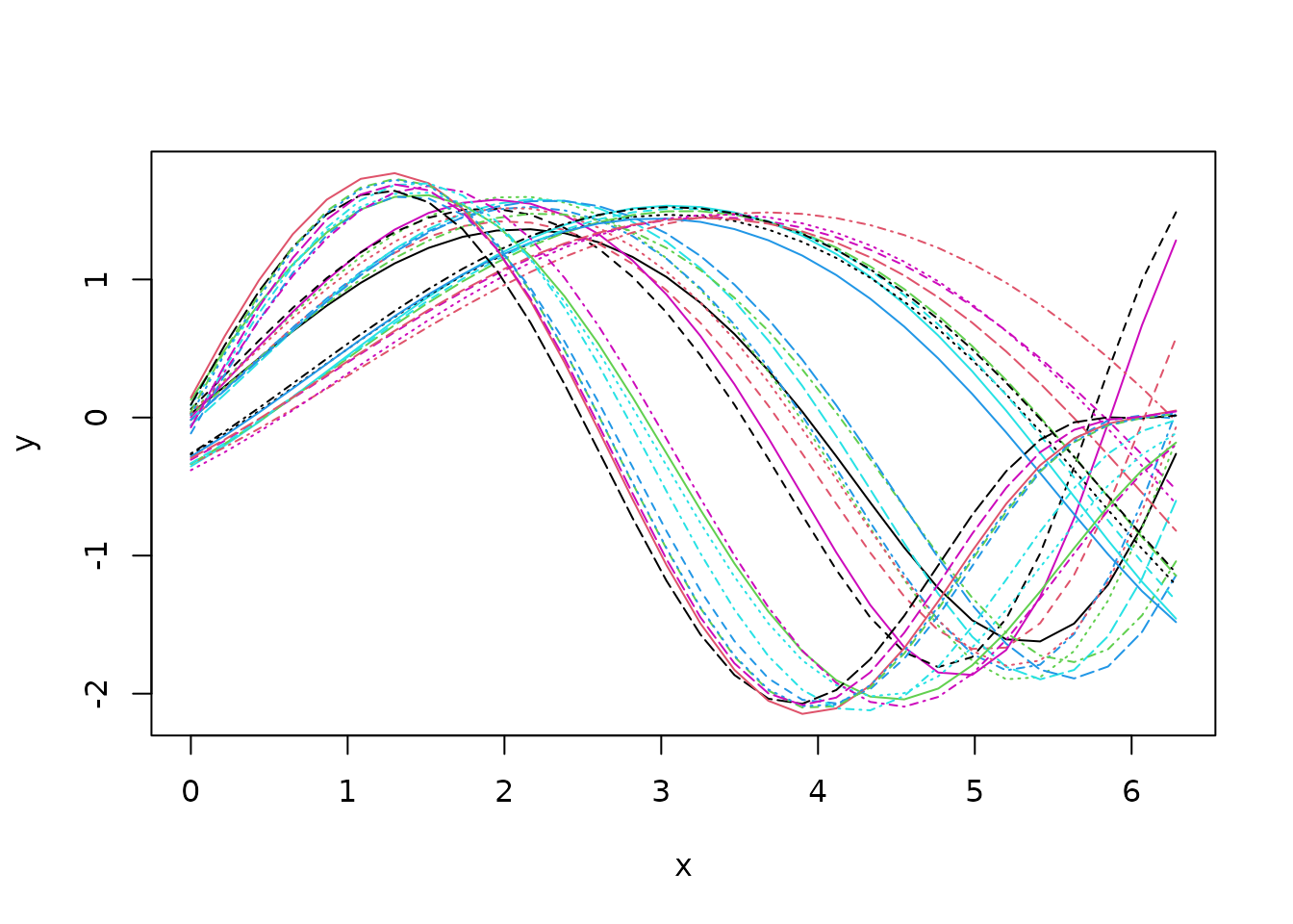
Looking at the data set, it seems that we shall expect \(3\) groups if we aim at clustering based on phase variability but probably only \(2\) groups if we search for a clustering structure based on amplitude variability.

HAC based on amplitude variability

We can perform HAC based on amplitude variability as follows:

out1 <- fdahclust(
  simulated30_sub$x,
  simulated30_sub$y,
  n_clusters = 2,
  centroid_type = "mean",
  warping_class = "affine",
  metric = "normalized_l2", 
  cluster_on_phase = FALSE
)

The fdahclust() function returns an object of class caps (for Clustering with Amplitude and Phase Separation) for which S3 specialized methods of ggplot2::autoplot() and graphics::plot() have been implemented.

For instance, we can visualize the original and aligned functional data set with:

plot(out1, type = "amplitude")

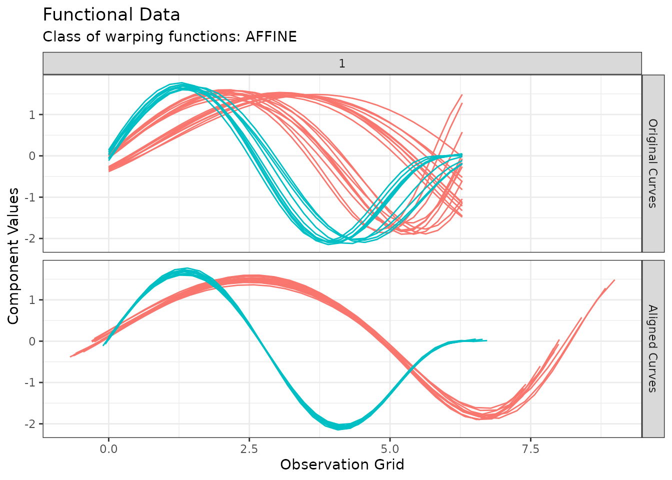
Or we can visualize the estimated warping functions with:

plot(out1, type = "phase")

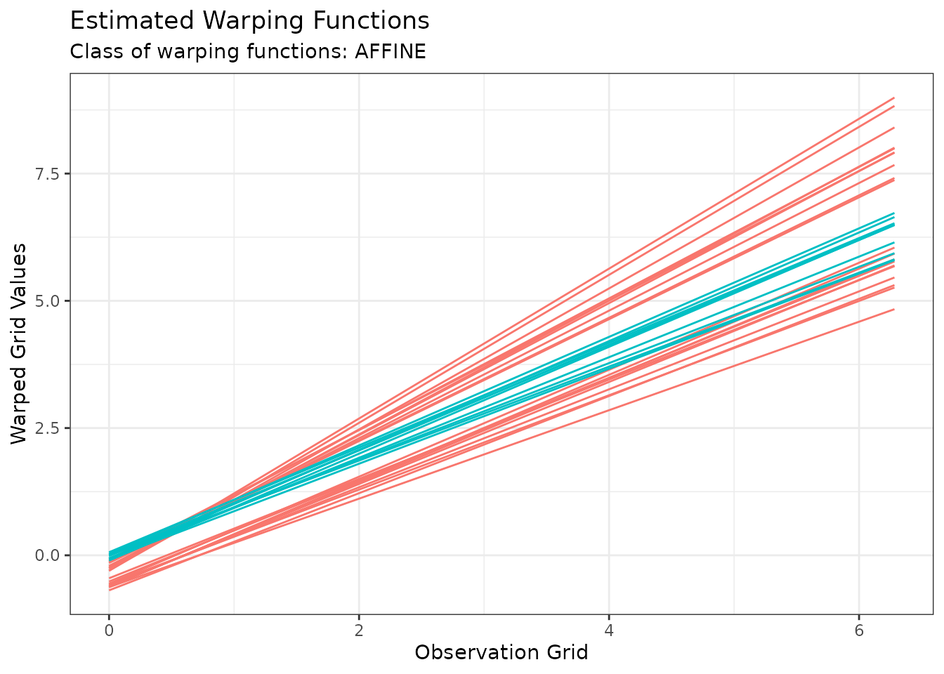
Or we can visualize the distribution of distances-to-center and silhouette values across observations with:

diagnostic_plot(out1)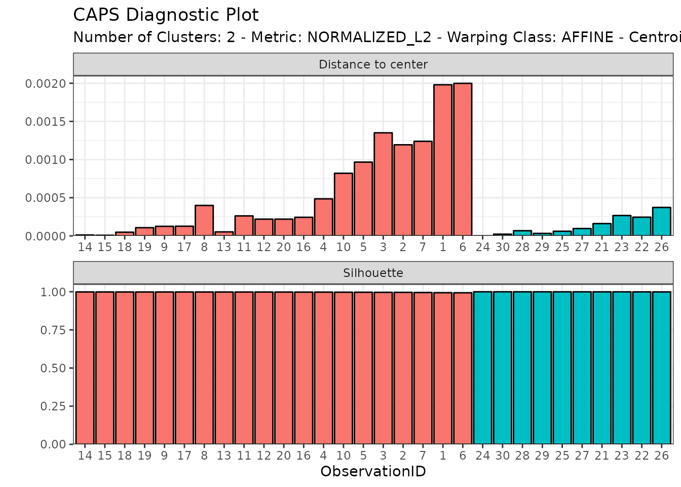

HAC based on phase variability

We can perform HAC based on phase variability only by switching the cluster_on_phase argument to TRUE:

out2 <- fdahclust(
  simulated30_sub$x,
  simulated30_sub$y,
  n_clusters = 3,
  centroid_type = "mean",
  warping_class = "affine",
  metric = "normalized_l2", 
  cluster_on_phase = TRUE
)

We can inspect the result as before:

plot(out2, type = "amplitude")

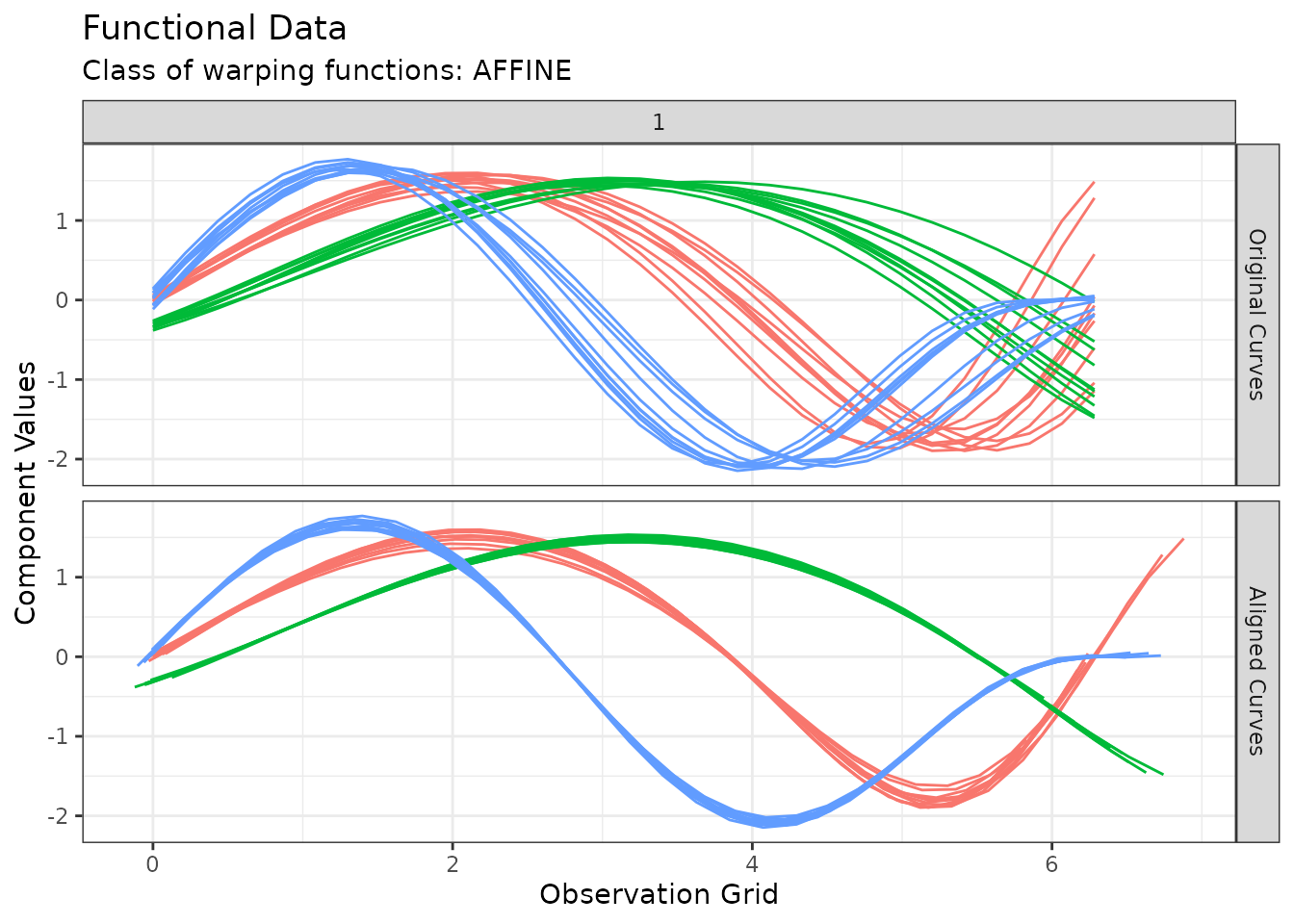
plot(out2, type = "phase")

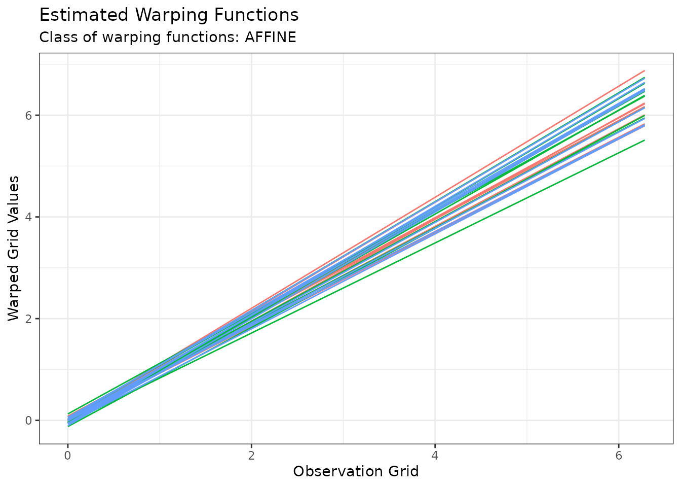
diagnostic_plot(out2)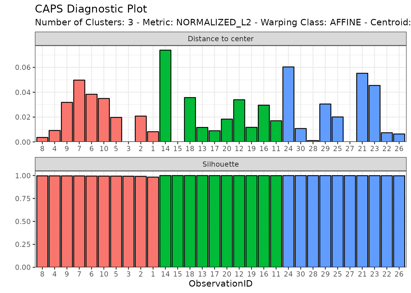

Choosing the number of clusters

The helper function compare_caps() can be used to get an intuition of the number of clusters that one should be looking for.

For example, we can generate data to help choosing the number of clusters when clustering on amplitude data:

ncores <- max(parallel::detectCores() - 1L, 1L)
plan(multisession, workers = ncores)
amplitude_data <- compare_caps(
  x = simulated30_sub$x, 
  y = simulated30_sub$y, 
  n_clusters = 1:5, 
  metric = "normalized_l2", 
  warping_class = c("none", "shift", "dilation", "affine"),
  clustering_method = "hclust-complete", 
  centroid_type = "mean", 
  cluster_on_phase = FALSE
)
plan(sequential)

In this example. we asked through the specification of the optional argument warping_class to use multiple warping classes and store the clustering results separately in the output for later comparison. Multiple choices can be also used for arguments clustering_method and centroid_type although in the above example we chose to focus on the HAC with complete linkage using the mean as centroid type. The metric argument must however be unique as we need to use the same metric among methods for later comparison.

The above code generates an object of class mcaps which has dedicated S3 specializations of ggplot2::autoplot() and graphics::plot() as well. These methods gain two extra optional arguments:

validation_criterion: A string specifying the validation criterion to be used for the comparison. Choices are "wss" or "silhouette". Defaults to "wss".
what: A string specifying the kind of information to display about the validation criterion. Choices are "mean" (which plots the mean values) or "distribution" (which plots the boxplots). Defaults to "mean".

For example, one can can visualize the mean WSS for all specified methods as:

plot(amplitude_data, validation_criterion = "wss", what = "mean")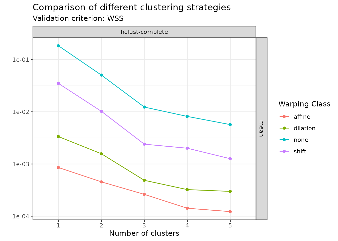

In this case, the plot clearly shows that among the set of warping classes that has been considered, one should use affine warping and search for \(2\) groups when the goal is to cluster based on amplitude variability.

Let us now perform the same analysis with the goal of clustering based on phase variability instead:

ncores <- max(parallel::detectCores() - 1L, 1L)
plan(multisession, workers = ncores)
phase_data <- compare_caps(
  x = simulated30_sub$x, 
  y = simulated30_sub$y, 
  n_clusters = 1:5, 
  metric = "normalized_l2", 
  warping_class = c("shift", "dilation", "affine"),
  clustering_method = "hclust-complete", 
  centroid_type = "mean", 
  cluster_on_phase = TRUE
)
plan(sequential)

plot(phase_data, validation_criterion = "wss", what = "mean")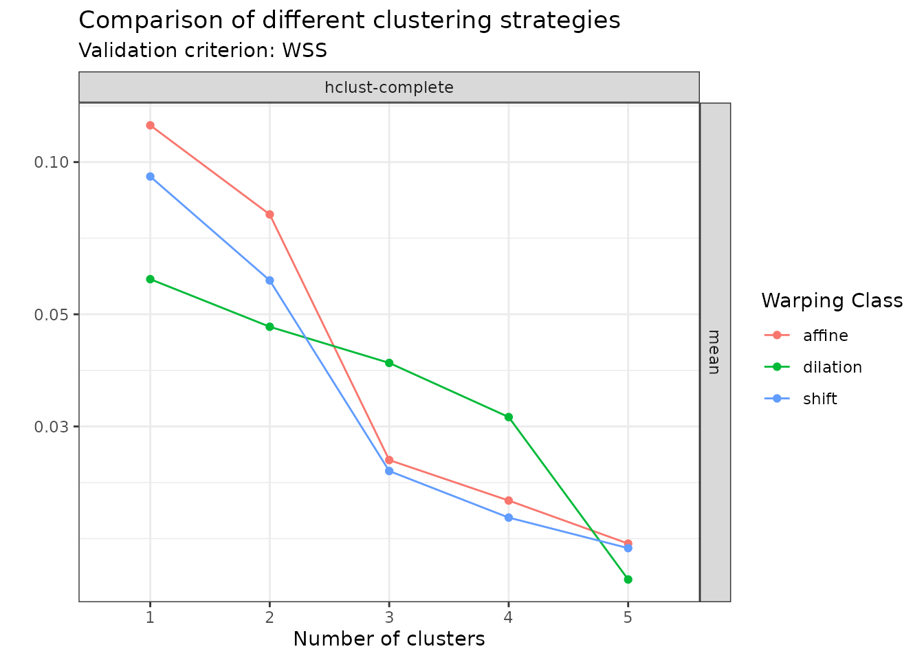

In this case, as expected by looking at the original data set, the plot suggests to search for \(3\) groups. What is even more interesting is that there is in this case no improvement in terms of WSS by going from the shift warping class to the affine warping class. This was also expected by looking at the original data set but it is nice that it is also reflected in the output diagnostic.