plot(mfdat)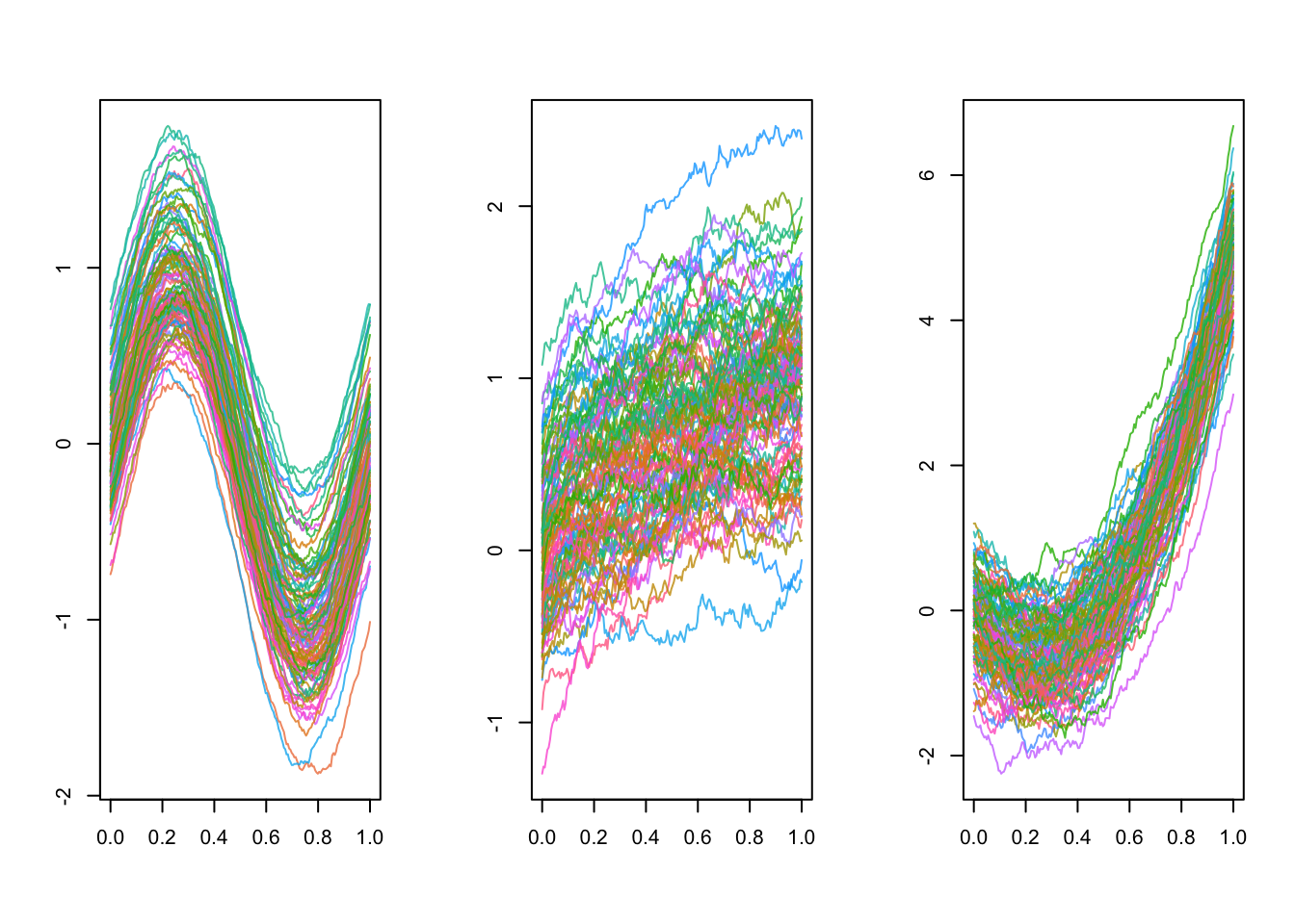
We have simulated 3D functional data for this lab that is provided in the Quarto document in the dat object.
The dat object is a list of size \(100\) containing \(100\) three-dimensional curves observed on a common grid of size \(200\) of the interval \([0, 1]\).
As a result, each element of the dat list is a \(3 \times 200\) matrix.
Here we focus on a subset of the data, the first \(21\) curves, which looks like:
plot(mfdat)
We can implement the Hausdorff distance between two curves as:
hausdorff_distance_vec <- function(x, y) {
  P <- ncol(x)
  dX <- 1:P |>
    purrr::map_dbl(\(p) {
      min(colSums((y - x[, p])^2))
    }) |>
    max()
  dY <- 1:P |>
    purrr::map_dbl(\(p) {
      min(colSums((x - y[, p])^2))
    }) |>
    max()
  sqrt(max(dX, dY))
}
This version exploits the vectorized nature of R to compute the Hausdorff distance via calls to colSums() and max(). Another version based on a double loop is provided by the following hausdorff_distance_for() function:
hausdorff_distance_for <- function(x, y) {
  P <- ncol(x)
  dX <- 0
  dY <- 0
  for (i in 1:P) {
    min_dist_x <- Inf
    min_dist_y <- Inf
    for (j in 1:P) {
      dist_x <- sum((y[, j] - x[, i])^2)
      if (dist_x < min_dist_x) {
        min_dist_x <- dist_x
      }
      dist_y <- sum((x[, j] - y[, i])^2)
      if (dist_y < min_dist_y) {
        min_dist_y <- dist_y
      }
    }
    if (min_dist_x > dX) {
      dX <- min_dist_x
    }
    if (min_dist_y > dY) {
      dY <- min_dist_y
    }
  }
  sqrt(max(dX, dY))
}
We can benchmark the two versions:
bm <- bench::mark(
  hausdorff_distance_vec(dat[[1]], dat[[2]]),
  hausdorff_distance_for(dat[[1]], dat[[2]])
)
Expression |
Median computation time |
Memory allocation |
|---|---|---|
| hausdorff_distance_vec(dat[[1]], dat[[2]]) | 2.02 ms | 2.7 MB |
| hausdorff_distance_for(dat[[1]], dat[[2]]) | 50.08 ms | 124.6 kB |
We conclude that the vectorized version is faster but has a huge memory footprint compared to the loop-based version. This means that the vectorized version is not suitable for even moderately large data sets.
Take a look at the documentation of the stats::dist() function to understand how to make an object of class dist.
We can exploit the previous functions to compute the pairwise distance matrix using the Hausdorff distance:
dist_r_v1 <- function(x, vectorized = FALSE) {
  hausdorff_distance <- if (vectorized)
    hausdorff_distance_vec
  else
    hausdorff_distance_for
  N <- length(x)
  out <- 1:(N - 1) |>
    purrr::map(\(i) {
      purrr::map_dbl((i + 1):N, \(j) {
        hausdorff_distance(x[[i]], x[[j]])
      })
    }) |>
    purrr::list_c()

  attributes(out) <- NULL
  attr(out, "Size") <- N
  lbls <- names(x)
  attr(out, "Labels") <- if (is.null(lbls)) 1:N else lbls
  attr(out, "Diag") <- FALSE
  attr(out, "Upper") <- FALSE
  attr(out, "method") <- "hausdorff"
  class(out) <- "dist"
  out
}
We can benchmark the two versions:
bm <- bench::mark(
  dist_r_v1(dat, vectorized = TRUE),
  dist_r_v1(dat, vectorized = FALSE)
)
Expression |
Median computation time |
Memory allocation |
|---|---|---|
| dist_r_v1(dat, vectorized = TRUE) | 0.48 s | 546.5 MB |
| dist_r_v1(dat, vectorized = FALSE) | 11.18 s | 3 kB |
We confirm that the vectorized version is not scalable to large datasets. Using it on the full dataset actually requires 12GB of memory! We will therefore focus on the loop-based version from now on.