Hausdorff Distance Matrix Computation

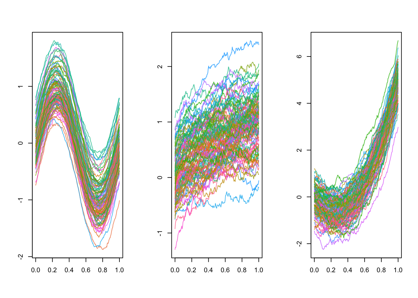
Solutions

Author

Aymeric Stamm

Published

September 27, 2024

Data & Goal

We have simulated 3D functional data for this lab that is provided in the Quarto document in the dat object.

The dat object is a list of size \(100\) containing \(100\) three-dimensional curves observed on a common grid of size \(200\) of the interval \([0, 1]\).

As a result, each element of the dat list is a \(3 \times 200\) matrix.

Here we focus on a subset of the data, the first \(21\) curves, which looks like:

plot(mfdat)

Objective

The goal is to implement a function similar to stats::dist() which computes the pairwise distance matrix on this functional dataset using the Hausdorff distance.

Hausdorff distance in R

We can implement the Hausdorff distance between two curves as:

hausdorff_distance_vec <- function(x, y) {
  P <- ncol(x)
  dX <- 1:P |>
    purrr::map_dbl(\(p) {
      min(colSums((y - x[, p])^2))
    }) |>
    max()
  dY <- 1:P |>
    purrr::map_dbl(\(p) {
      min(colSums((x - y[, p])^2))
    }) |>
    max()
  sqrt(max(dX, dY))
}

This version exploits the vectorized nature of R to compute the Hausdorff distance via calls to colSums() and max(). Another version based on a double loop is provided by the following hausdorff_distance_for() function:

hausdorff_distance_for <- function(x, y) {
  P <- ncol(x)
  dX <- 0
  dY <- 0
  for (i in 1:P) {
    min_dist_x <- Inf
    min_dist_y <- Inf
    for (j in 1:P) {
      dist_x <- sum((y[, j] - x[, i])^2)
      if (dist_x < min_dist_x) {
        min_dist_x <- dist_x
      }
      dist_y <- sum((x[, j] - y[, i])^2)
      if (dist_y < min_dist_y) {
        min_dist_y <- dist_y
      }
    }
    if (min_dist_x > dX) {
      dX <- min_dist_x
    }
    if (min_dist_y > dY) {
      dY <- min_dist_y
    }
  }
  sqrt(max(dX, dY))
}

We can benchmark the two versions:

bm <- bench::mark(
  hausdorff_distance_vec(dat[[1]], dat[[2]]),
  hausdorff_distance_for(dat[[1]], dat[[2]])
)

Expression	Median computation time	Memory allocation
hausdorff_distance_vec(dat[[1]], dat[[2]])	2.02 ms	2.7 MB
hausdorff_distance_for(dat[[1]], dat[[2]])	50.08 ms	124.6 kB

We conclude that the vectorized version is faster but has a huge memory footprint compared to the loop-based version. This means that the vectorized version is not suitable for even moderately large data sets.

Pairwise distance matrix in R

dist objects

Take a look at the documentation of the stats::dist() function to understand how to make an object of class dist.

We can exploit the previous functions to compute the pairwise distance matrix using the Hausdorff distance:

dist_r_v1 <- function(x, vectorized = FALSE) {
  hausdorff_distance <- if (vectorized) 
    hausdorff_distance_vec
  else 
    hausdorff_distance_for
  N <- length(x)
  out <- 1:(N - 1) |>
    purrr::map(\(i) {
      purrr::map_dbl((i + 1):N, \(j) {
        hausdorff_distance(x[[i]], x[[j]])
      })
    }) |>
    purrr::list_c()

  attributes(out) <- NULL
  attr(out, "Size") <- N
  lbls <- names(x)
  attr(out, "Labels") <- if (is.null(lbls)) 1:N else lbls
  attr(out, "Diag") <- FALSE
  attr(out, "Upper") <- FALSE
  attr(out, "method") <- "hausdorff"
  class(out) <- "dist"
  out
}

We can benchmark the two versions:

bm <- bench::mark(
  dist_r_v1(dat, vectorized = TRUE),
  dist_r_v1(dat, vectorized = FALSE)
)

Expression	Median computation time	Memory allocation
dist_r_v1(dat, vectorized = TRUE)	0.48 s	546.5 MB
dist_r_v1(dat, vectorized = FALSE)	11.18 s	3 kB

Memory footprint

We confirm that the vectorized version is not scalable to large datasets. Using it on the full dataset actually requires 12GB of memory! We will therefore focus on the loop-based version from now on.

futureverse

Parallelize outer loop

dist_r_v2 <- function(x) {
  N <- length(x)
  out <- 1:(N - 1) |>
    furrr::future_map(\(i) {
      purrr::map_dbl((i + 1):N, \(j) {
        hausdorff_distance_for(x[[i]], x[[j]])
      })
    }) |>
    purrr::list_c()

  attributes(out) <- NULL
  attr(out, "Size") <- N
  lbls <- names(x)
  attr(out, "Labels") <- if (is.null(lbls)) 1:N else lbls
  attr(out, "Diag") <- FALSE
  attr(out, "Upper") <- FALSE
  attr(out, "method") <- "hausdorff"
  class(out) <- "dist"
  out
}

Tweaking the chunk size

dist_r_v3 <- function(x) {
  N <- length(x)
  out <- 1:(N - 1) |>
    furrr::future_map(\(i) {
      purrr::map_dbl((i + 1):N, \(j) {
        hausdorff_distance_for(x[[i]], x[[j]])
      })
    }, .options = furrr::furrr_options(chunk_size = 1)) |>
    purrr::list_c()

  attributes(out) <- NULL
  attr(out, "Size") <- N
  lbls <- names(x)
  attr(out, "Labels") <- if (is.null(lbls)) 1:N else lbls
  attr(out, "Diag") <- FALSE
  attr(out, "Upper") <- FALSE
  attr(out, "method") <- "hausdorff"
  class(out) <- "dist"
  out
}

Nested plan

dist_r_v4 <- function(x) {
  N <- length(x)
  out <- 1:(N - 1) |>
    furrr::future_map(\(i) {
      furrr::future_map_dbl((i + 1):N, \(j) {
        hausdorff_distance_for(x[[i]], x[[j]])
      })
    }, .options = furrr::furrr_options(chunk_size = 1)) |>
    purrr::list_c()

  attributes(out) <- NULL
  attr(out, "Size") <- N
  lbls <- names(x)
  attr(out, "Labels") <- if (is.null(lbls)) 1:N else lbls
  attr(out, "Diag") <- FALSE
  attr(out, "Upper") <- FALSE
  attr(out, "method") <- "hausdorff"
  class(out) <- "dist"
  out
}

Convert to single loop

dist_r_v5 <- function(x) {
  N <- length(x)
  K <- N * (N - 1) / 2
  out <- furrr::future_map_dbl(1:K, \(k) {
    k <- k - 1
    i <- N - 2 - floor(sqrt(-8 * k + 4 * N * (N - 1) - 7) / 2.0 - 0.5);
    j <- k + i + 1 - N * (N - 1) / 2 + (N - i) * ((N - i) - 1) / 2;
    i <- i + 1
    j <- j + 1
    hausdorff_distance_for(x[[i]], x[[j]])
  })
  attributes(out) <- NULL
  attr(out, "Size") <- N
  lbls <- names(x)
  attr(out, "Labels") <- if (is.null(lbls)) 1:N else lbls
  attr(out, "Diag") <- FALSE
  attr(out, "Upper") <- FALSE
  attr(out, "method") <- "hausdorff"
  class(out) <- "dist"
  out
}

C++ implementation

The fact that the dist function takes a list of matrices as input can be handled by {Rcpp}. However, there is no threadsafe wrapper for lists due to the fact that they can store objects of different types and thus cannot be serialized.

We therefore use a vector representation for an \(L\)-dimensional curve observed on a grid of \(P\) points. The vector is of length \(L \times N\). This allows the entire data set to be passed as a single matrix \(X\) to the C++ function where the \(i\)-th row reads:

\[ x_i^{(1)}(t_1), \dots, x_i^{(1)}(t_P), x_i^{(2)}(t_1), \dots, x_i^{(2)}(t_P), \dots, x_i^{(L)}(t_1), \dots, x_i^{(L)}(t_P). \]

#include <Rcpp.h>

// // [[Rcpp::plugins(openmp)]] // Uncomment on Windows and Linux

// [[Rcpp::depends(RcppParallel)]]
#include <RcppParallel.h>

// [[Rcpp::export]]
double hausdorff_distance_cpp(Rcpp::NumericVector x, Rcpp::NumericVector y,
                              unsigned int dimension = 1)
{
  unsigned int numDimensions = dimension;
  unsigned int numPoints = x.size() / numDimensions;

  double dX = 0.0;
  double dY = 0.0;

  for (unsigned int i = 0;i < numPoints;++i)
  {
    double min_dist_x = std::numeric_limits<double>::infinity();
    double min_dist_y = std::numeric_limits<double>::infinity();

    for (unsigned int j = 0;j < numPoints;++j)
    {
      double dist_x = 0.0;
      double dist_y = 0.0;

      for (unsigned int k = 0;k < numDimensions;++k)
      {
        unsigned int index_i = k * numPoints + i;
        unsigned int index_j = k * numPoints + j;
        dist_x += std::pow(x[index_i] - y[index_j], 2);
        dist_y += std::pow(y[index_i] - x[index_j], 2);
      }
      min_dist_x = std::min(min_dist_x, dist_x);
      min_dist_y = std::min(min_dist_y, dist_y);
    }

    dX = std::max(dX, min_dist_x);
    dY = std::max(dY, min_dist_y);
  }

  return std::sqrt(std::max(dX, dY));
}

double hausdorff_distance_cpp(RcppParallel::RMatrix<double>::Row x,
                              RcppParallel::RMatrix<double>::Row y,
                              unsigned int dimension = 1)
{
  unsigned int numDimensions = dimension;
  unsigned int numPoints = x.size() / numDimensions;

  double dX = 0.0;
  double dY = 0.0;

  for (unsigned int i = 0;i < numPoints;++i)
  {
    double min_dist_x = std::numeric_limits<double>::infinity();
    double min_dist_y = std::numeric_limits<double>::infinity();

    for (unsigned int j = 0;j < numPoints;++j)
    {
      double dist_x = 0.0;
      double dist_y = 0.0;

      for (unsigned int k = 0;k < numDimensions;++k)
      {
        unsigned index_i = k * numPoints + i;
        unsigned index_j = k * numPoints + j;
        dist_x += std::pow(x[index_i] - y[index_j], 2);
        dist_y += std::pow(y[index_i] - x[index_j], 2);
      }

      min_dist_x = std::min(min_dist_x, dist_x);
      min_dist_y = std::min(min_dist_y, dist_y);
    }

    dX = std::max(dX, min_dist_x);
    dY = std::max(dY, min_dist_y);
  }

  return std::sqrt(std::max(dX, dY));
}

Rcpp::NumericMatrix listToMatrix(Rcpp::List x)
{
  unsigned int nrows = x.size();
  unsigned int ncols = Rcpp::as<Rcpp::NumericVector>(x[0]).size();
  Rcpp::NumericMatrix out(nrows, ncols);
  Rcpp::NumericMatrix workMatrix;
  Rcpp::NumericVector row;

  for (unsigned int i = 0;i < nrows;++i)
  {
    workMatrix = Rcpp::as<Rcpp::NumericMatrix>(x[i]);
    workMatrix = Rcpp::transpose(workMatrix);
    row = Rcpp::as<Rcpp::NumericVector>(workMatrix);
    std::copy(row.begin(), row.end(), out.row(i).begin());
  }

  return out;
}

Rcpp::NumericVector dist_cpp_omp(Rcpp::NumericMatrix x,
                                 unsigned int dimension = 1,
                                 unsigned int ncores = 1)
{
  unsigned int N = x.nrow();
  unsigned int K = N * (N - 1) / 2;
  Rcpp::NumericVector out(K);
  RcppParallel::RMatrix<double> xSafe(x);
  RcppParallel::RVector<double> outSafe(out);

#ifdef _OPENMP
  #pragma omp parallel for num_threads(ncores)
#endif
  for (unsigned int k = 0;k < K;++k)
  {
    unsigned int i = N - 2 - std::floor(std::sqrt(-8 * k + 4 * N * (N - 1) - 7) / 2.0 - 0.5);
    unsigned int j = k + i + 1 - N * (N - 1) / 2 + (N - i) * ((N - i) - 1) / 2;
    outSafe[k] = hausdorff_distance_cpp(xSafe.row(i), xSafe.row(j), dimension);
  }

  out.attr("Size") = N;
  out.attr("Labels") = Rcpp::seq(1, N);
  out.attr("Diag") = false;
  out.attr("Upper") = false;
  out.attr("method") = "hausdorff";
  out.attr("class") = "dist";
  return out;
}

// [[Rcpp::export]]
Rcpp::NumericVector dist_cpp_omp(Rcpp::List x,
                                 unsigned int dimension = 1,
                                 unsigned int ncores = 1)
{
  Rcpp::NumericMatrix xMatrix = listToMatrix(x);
  return dist_cpp_omp(xMatrix, dimension, ncores);
}

struct HausdorffDistanceComputer : public RcppParallel::Worker
{
  const RcppParallel::RMatrix<double> m_SafeInput;
  RcppParallel::RVector<double> m_SafeOutput;
  unsigned int m_Dimension;

  HausdorffDistanceComputer(const Rcpp::NumericMatrix x,
                    Rcpp::NumericVector out,
                    unsigned int dimension)
    : m_SafeInput(x), m_SafeOutput(out), m_Dimension(dimension) {}

  void operator()(std::size_t begin, std::size_t end)
  {
    unsigned int N = m_SafeInput.nrow();
    for (std::size_t k = begin;k < end;++k)
    {
      unsigned int i = N - 2 - std::floor(std::sqrt(-8 * k + 4 * N * (N - 1) - 7) / 2.0 - 0.5);
      unsigned int j = k + i + 1 - N * (N - 1) / 2 + (N - i) * ((N - i) - 1) / 2;
      m_SafeOutput[k] = hausdorff_distance_cpp(m_SafeInput.row(i), m_SafeInput.row(j), m_Dimension);
    }
  }
};

Rcpp::NumericVector dist_rcppparallel(Rcpp::NumericMatrix x,
                                      unsigned int dimension = 1,
                                      unsigned int ncores = 1)
{
  unsigned int N = x.nrow();
  unsigned int K = N * (N - 1) / 2;
  Rcpp::NumericVector out(K);
  HausdorffDistanceComputer hausdorffDistance(x, out, dimension);
  RcppParallel::parallelFor(0, K, hausdorffDistance, 1, ncores);
  out.attr("Size") = x.nrow();
  out.attr("Labels") = Rcpp::seq(1, x.nrow());
  out.attr("Diag") = false;
  out.attr("Upper") = false;
  out.attr("method") = "hausdorff";
  out.attr("class") = "dist";
  return out;
}

// [[Rcpp::export]]
Rcpp::NumericVector dist_rcppparallel(Rcpp::List x,
                                      unsigned int dimension = 1,
                                      unsigned int ncores = 1)
{
  Rcpp::NumericMatrix xMatrix = listToMatrix(x);
  return dist_rcppparallel(xMatrix, dimension, ncores);
}

The hausdorff_distance_cpp() function implements the Hausdorff distance between two curves, where a curve is stored as a vector as described in the beginning of the section. The function therefore takes an additional optional argument to specify the dimension of the curve. The function has two implementations with different input types (Rcpp::NumericVector and RcppParallel::RMatrix<double>::Row). The latter is used to parallelize the computation using the thread-safe accessor to vectors. Only the former is exported to R.

The listToMatrix() function is used to convert a list of matrices to a single matrix that stores the sample of curves in a format that can be passed to the dist_cpp_omp() and dist_rcppparallel() functions in a thread-safe manner.

The dist_cpp_omp() and dist_rcppparallel() functions compute the Hausdorff distance between all pairs of curves in the sample. The former uses OpenMP to parallelize the computation, while the latter uses {RcppParallel}. Both functions have two implementations with different input types (Rcpp::NumericMatrix and Rcpp::List). The former can be wrapped with the tread-safe accessor to matrices, while the latter is the one that is exported to R and internally uses the listToMatrix() function to convert the input list to a matrix.

The dist_rcppparallel() function parallelizes the computations via the RcppParallel::parallelFor() function, which requires a RcppParallel::Worker object. The HausdorffDistanceComputer class inherits from the RcppParallel::Worker class and is used to implement exactly what a single worker should do.

Benchmark

library(future)

bm <- bench::mark(
  sequential = dist_r_v1(dat, vectorized = FALSE),
  outer = {
    plan(multisession, workers = 4L)
    out <- dist_r_v2(dat)
    plan(sequential)
    out
  },
  chunksize = {
    plan(multisession, workers = 4L)
    out <- dist_r_v3(dat)
    plan(sequential)
    out
  },
  nested = {
    plan(list(
      tweak(multisession, workers = 2L),
      tweak(multisession, workers = I(2L))
    ))
    out <- dist_r_v4(dat)
    plan(sequential)
    out
  },
  singleloop = {
    plan(multisession, workers = 4L)
    out <- dist_r_v5(dat)
    plan(sequential)
    out
  },
  openmp1 = dist_cpp_omp(dat, dimension = 3L, ncores = 1L),
  openmp4 = dist_cpp_omp(dat, dimension = 3L, ncores = 4L),
  rcppparallel1 = dist_rcppparallel(dat, dimension = 3L, ncores = 1L),
  rcppparallel4 = dist_rcppparallel(dat, dimension = 3L, ncores = 4L)
)

Comparison of different implementations
The computation time is given in milliseconds and the memory allocation in bytes.
Language	Expression	Median computation time	Memory allocation
R	sequential	11,291.89 ms	278.4 kB
R	outer	5,328.50 ms	6.9 MB
R	chunksize	3,711.79 ms	27.6 MB
R	nested	4,399.25 ms	17.4 MB
R	singleloop	3,700.71 ms	7 MB
C++	openmp1	24.25 ms	204.4 kB
C++	openmp4	6.34 ms	209.1 kB
C++	rcppparallel1	24.36 ms	204.4 kB
C++	rcppparallel4	6.44 ms	209.1 kB

Interpretation

General observation. Using C++ is much faster than using R. This is in particular due to never copying the data. It also provides linear speed-up as expected.

R implementation. The original Hausdorff distance implementation has a double loop.

The outer loop generates unbalanced chunks, which is not optimal (outer entry).
Load balancing is better with a fixed chunk size of 1 (chunksize entry).
Using nested parallelization does not help (nested entry) achieves intermediate results. It is better than the outer loop but worse than the fixed chunk size.
Transforming the original double loop into a single loop (singleloop entry) is as fast as parallelizing the outer loop using a chunk size of 1 (singleloop entry) but its memory allocation is much lower. This is because, when the chunk size is 1, a future is created for each iteration of the loop, and the whole data is copied for each future. In contrast, the single loop version submits a single future per worker which creates less copies of the data.
In general, playing with chunk size and nested parallelization generates more future objects and copies the data more often, which increases memory allocation.