fdacluster

An R package for joint clustering and alignment of functional data

L. Bellanger, A. Stamm

Department of Mathematics Jean Leray, UMR CNRS 6629, Nantes University, France

L.M. Sangalli, P. Secchi, S. Vantini

MOX - Department of Mathematics, Politecnico di Milano, Italy

2023-06-22

Title explanation

Clustering

• Unlabeled data: observations are not assigned to pre-existing groups;
• Goal: group together individuals or observations that share common features while ensuring the following property:
  • observations within a group must be as similar as possible,
  • observations between groups (belonging to different groups) must be as different as possible.

Clustering methods

Centroid-based clustering

Clusters are represented by a central value or centroid. This centroid might not necessarily be one of the observations. These methods (e.g. k-means) operate in an iterative fashion in which the notion of similarity is derived by how close an observation is to the centroid of the cluster.

Hierarchical clustering

Observations that are closer in the data space are more related (similar) than observations that are far from each other. Clusters are formed by connecting observations according to their distance and clusters are allowed to be merged or splitted according to a cluster-based distance.

Density-based clustering

Search the data space for areas of high density of observations (e.g. DBSCAN). Clusters are defined as the areas of higher density within the data space compared to other regions. Observations in the sparse areas are usually considered to be noise and/or border points.

A common ingredient

All methods but model-based rely on the ability to quantify closeness / distance between observations.

Functional data - Visual definition

Data source: Berkeley Growth Study data (Tuddenham and Snyder 1954; Ramsay and Silverman 2006)

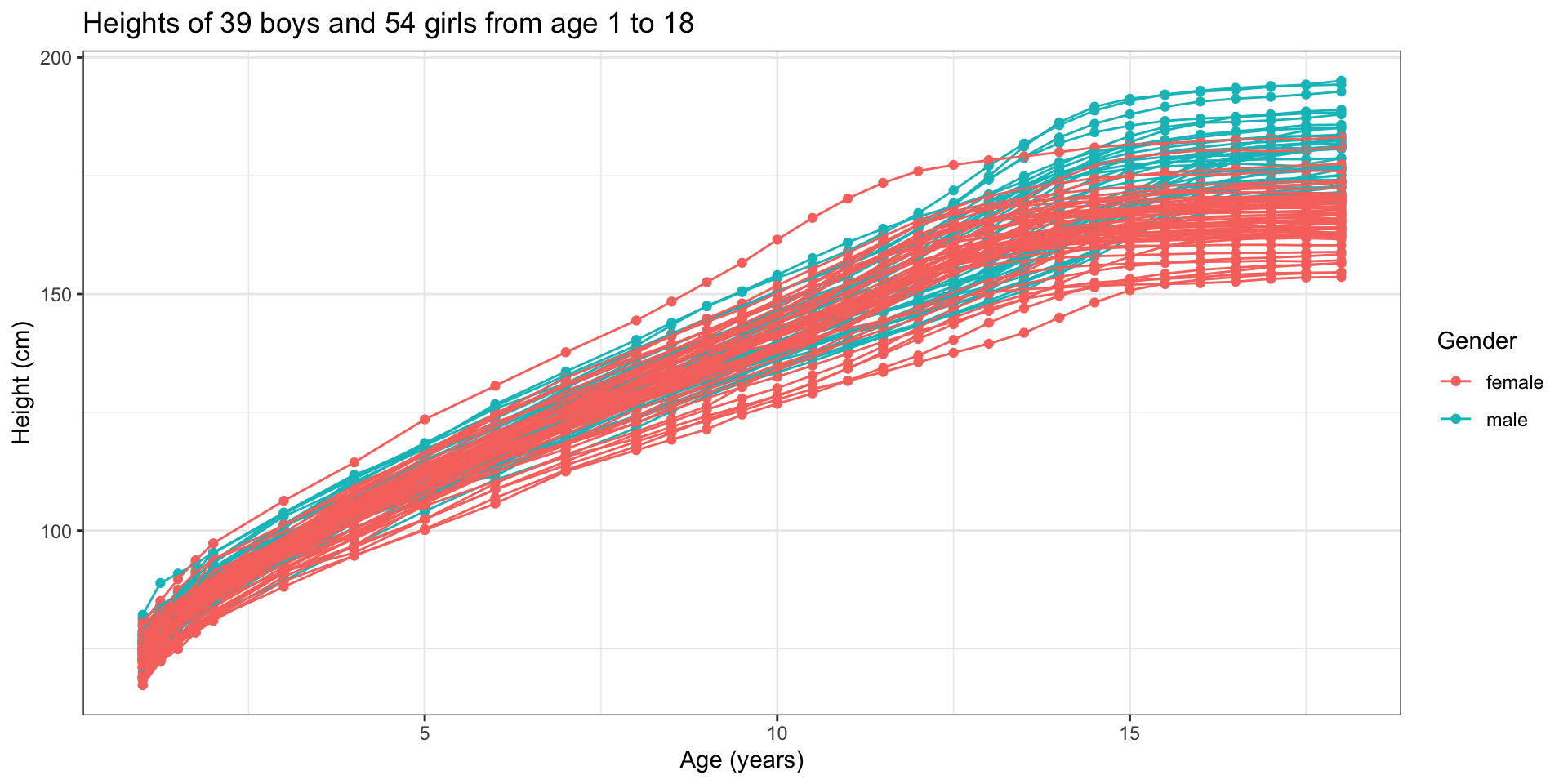
Functional data - Derivatives

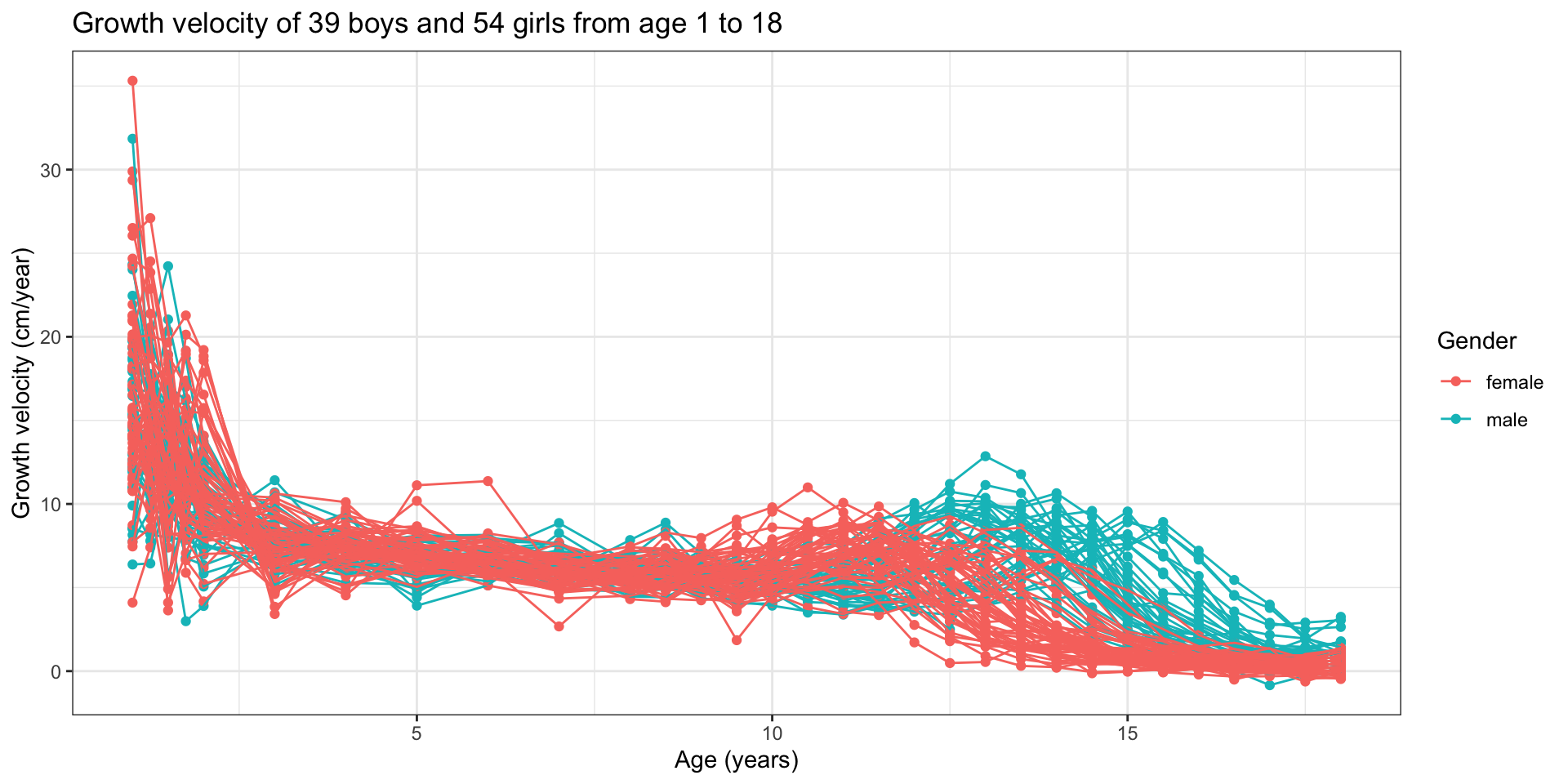
What if we did not know gender membership?

• Common peak of growth velocity shortly after birth
• Another smaller peak at puberty occurring:
  • At different ages for girls and for boys;
  • At different ages for each individual.

Functional clustering

Functional data - Notations

• We consider a random variable \(X\) which takes values in \(F = \{ f: \mathcal{D} \to \mathcal{M} \}\).
• The domain \(\mathcal{D}\) of the functions in \(F\) is a subset of \(\mathbb{R}\). Typically \(\mathcal{D} = \mathbb{R}\) or \(\mathcal{D} = [a, b]\).
• The co-domain \(\mathcal{M}\) of the functions in \(F\) can be univariate or multivariate and can be either a Euclidean space or more generally a manifold. Typically, \(\mathcal{M} = \mathbb{R}^p\).
• The space \(F\) is equipped with a metric \(d\) so that \((F, d)\) is a metric space.

Functional data - A simpler example

Data source: Sangalli et al. (2010).

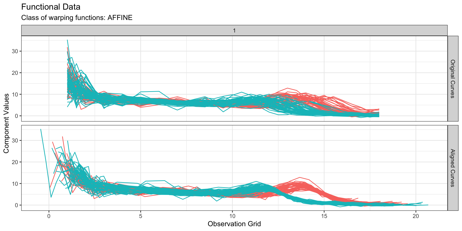
Functional data - Clustering

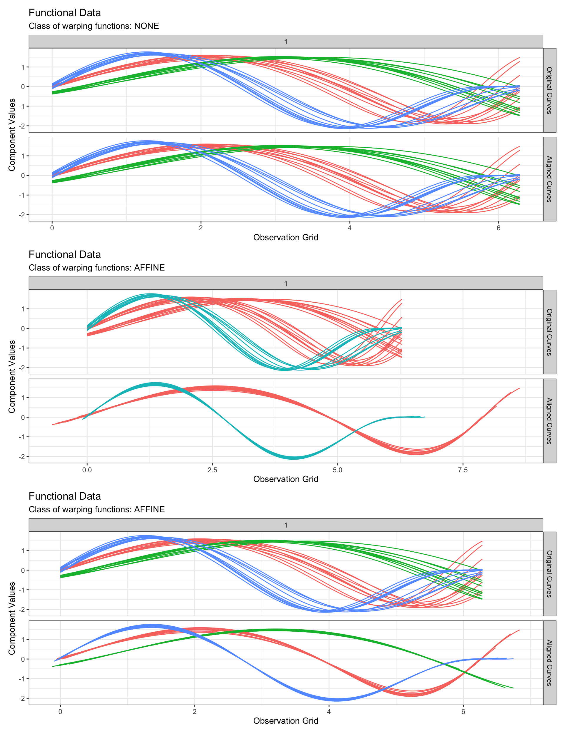
Solution 1: \[ \begin{cases} d_A^2(f, g) = d^2(f, g) \\ d_C^2(f, g) = d_A^2(f, g) \end{cases} \]

Solutions 2 & 3: \[ \begin{cases} d_A^2(f, g) = \min_{h \in W} d^2(f \circ h, g) \\ d_C^2(f, g) = d_A^2(f, g) \end{cases} \]

\[ \begin{cases} d_A^2(f, g) = \min_{h \in W} d^2(f \circ h, g) \\ d_C^2(f, g) = \int_{\mathcal{D}} \left[ h^\star(t) - t \right]^2 dt \\ \end{cases} \] with \(h^\star(t) = \arg \min_{h \in W} d^2(f \circ h, g)\).

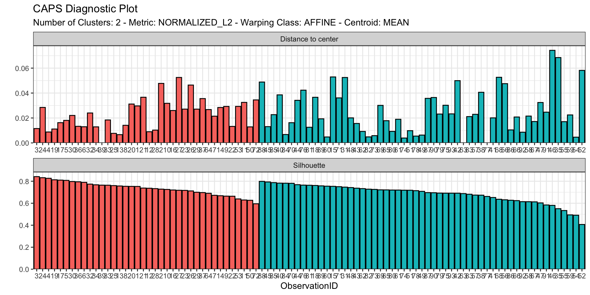
Registration of curves

The following properties on the functional space \(F\), its metric \(d\) and the set \(W\) of warping functions considered for curve registration must be satisfied for a mathematically consistent registration setup (Vantini 2012):

1. \(F = \{ f: \mathcal{D} \to \mathcal{M} \}\) is a metric space equipped with a metric \(d: F \times F \to \mathbb{R}^+\);

2. \(W\) is a subgroup — with respect to ordinary composition \(\circ\) — of the group of the continuous automorphisms of \(\mathcal{D}\);

3. \(\forall f \in F\) and \(\forall h \in W\), we have that \(f \circ h \in F\);

4. Given any couple of elements \(f_1, f_2 \in F\) and an element \(h \in W\), the distance between \(f_1\) and \(f_2\) is invariant under the composition of \(f_1\) and \(f_2\) with \(h\), i.e.:

\[ d(f_1, f_2) = d(f_1 \circ h, f_2 \circ h). \]

We will refer to this property as \(W\)-invariance of \(d\).

The case \(\mathcal{D} = \mathbb{R}\)

In this situation, it is not possible to perform registration over \(\mathbb{R}\) and most of the time we use \(W\) to be the set of affine warping functions i.e. \(W = \{ h: h(t) = at+b \}\).

In this setting, it is tempting to equip \(F\) with the \(L^2\)-distance: \[ d_{L^2}^2(f, g) = \int_\mathbb{R} \left\| f(t) - g(t) \right\|_{\mathbb{R}^p}^2 dt. \]

The \(L^2\)-distance is however not affine-invariant:

\[ d_{L^2}^2(f \circ h, g \circ h) = \frac{1}{a} d_{L^2}^2(f, g) \]

A proper normalization can make it affine-invariant such as: \[ d(f, g) = \frac{d_{L^2}(f, g)}{\| f \|_{L^2} + \| g \|_{L^2}} \]

The case \(\mathcal{D} = [a, b]\)

In this situation, it is possible to perform registration over the set \(W\) of all boundary-preserving warping functions by using the square-root slope function (SRSF) framework (Tucker, Wu, and Srivastava 2013) under the assumption that all functions \(f \in F\) are absolutely continuous. In this case, the SRSF of a function \(f \in F\) which reads:

\[ \begin{array}{rccl} q_f : & \mathbb{R} & \to & \mathbb{R}^p \\ & t & \mapsto & \frac{\dot{f}(t)}{\sqrt{ \| \dot{f}(t) \|_{\mathbb{R}^p} }}, \end{array} \] is square-integrable and thus belong to \(L^2([a,b], \mathbb{R}^p)\).

We can therefore define: \[ d(f, g) = d_{L^2}(q_f, q_g), \] and one can show that \(d\) is invariant under any boundary-preserving warping.

Funct. \(k\)-means (Sangalli et al. 2010)

Initialization

Choose \(k\) initial observations as cluster centroids.

Align observations

Perform registration of all observed curves on each cluster centroid.

Assign observations to closest centroid

Assign each observed curve to the cluster with smallest distance to its center. This involves solving a constrained mixed integer and linear programming problem to ensure that no requested cluster will be empty.

Update cluster centroids

Recompute each cluster centroid given the newly assigned observations. Since the solution to the registration problem is not unique, the unique centroid is computed according to recommendations in Vantini (2012) to minimize total variation. If \(f_0\) is a computed centroid, then define the cluster centroid as \[ \widehat{f_0} = \arg \min_{f \in [f_0]} \sum_{i=1}^n d^2(f_i, f), \] which is achieved for some warping function \(h^\star\) which needs to be further applied to all observations in that cluster.

Funct. hierarchical clustering

Distance matrix computation

Compute the matrix \(D\) of pairwise distances between curves minimizing over the selected class \(W\) of warping functions.

Dendrogram computation

Apply traditional approaches to hierarchical clustering on \(D\) (either agglomerative or divisive) to build a hierarchy of possible clustering partitions of the data (dendrogram).

Assign observations to clusters

• Cut the dendrogram to form \(k\) clusters and, in each cluster;
• Register all curves to centroid via funct. \(1\)-mean clustering.

Update distance matrix

Update the distance matrix \(D\) using the registered curves from previous step with no further registration. This is used for final calculations of WSS and silhouettes.

Functional DBSCAN

Adapting DBSCAN to functional data follows the same principles.

The R package fdacluster

On CRAN (or almost)

You can install the official version from CRAN via:

install.packages("fdacluster")

or you can opt to install the development version from GitHub with:

# install.packages("remotes")
remotes::install_github("astamm/fdacluster")

Website

https://astamm.github.io/fdacluster/index.html

Test it out now!

If you want to test the package right now, use the development version.

Features

1. A dedicated S3 class for storing results of clustering with amplitude and phase separation;

2. Implementations of k-means, HAC and DBSCAN methods for functional data;

3. Built-in parallelization;

4. Tools for comparing various clustering strategies:

   • compare_caps(): generates an object of class mcaps() containing caps objects for several clustering strategies;
   • plot() and autoplot() S3 specialized methods for mcaps objects.

5. Integration within the R fda landscape: input grids and curves can be

   • vectors, matrices, arrays; or,
   • fd objects from the fda package; or,
   • funData or multiFunData objects from the funData package.

Built-in parallelization

• Achieved via the futureverse framework;
• Possibility of displaying a progress bar.

library(future)
library(progressr)
handlers("rstudio") # Defines RStudio progress bar style
plan(multisession, workers = parallelly::availableCores(omit = 1)) # Turns ON parallelization
with_progress(
  # User-defined code for clustering
  out1 <- fdahclust(
    x = x,
    y = t(y1),
    n_clusters = 2,
    warping_class = "affine",
    cluster_on_phase = TRUE
  )
)
plan(sequential) # Turns OFF parallelization

The caps class

List of 14
 $ original_curves    : num [1:93, 1, 1:31] 12.44 18.13 12.02 16.92 8.51 ...
 $ original_grids     : num [1:93, 1:31] 1 1 1 1 1 1 1 1 1 1 ...
 $ aligned_grids      : num [1:93, 1:31] 1.383 1.646 2.078 0.878 1.941 ...
 $ center_curves      : num [1:2, 1, 1:31] 18.8 19.5 15.2 16.8 11.7 ...
 $ center_grids       : num [1:2, 1:31] 0.469 -0.199 1.1 0.493 1.732 ...
 $ n_clusters         : num 2
 $ memberships        : Named int [1:93] 1 1 1 1 1 1 1 1 1 1 ...
  ..- attr(*, "names")= chr [1:93] "1" "2" "3" "4" ...
 $ distances_to_center: num [1:93] 0.0164 0.0526 0.027 0.0151 0.0164 ...
 $ silhouettes        : num [1:93] 0.721 0.783 0.855 0.845 0.805 ...
 $ amplitude_variation: num 0.094
 $ total_variation    : num 0.167
 $ n_iterations       : num 0
 $ call_name          : chr "fdahclust"
 $ call_args          :List of 17
  ..$ x                           : symbol x
  ..$ y                           : language t(y1)
  ..$ n_clusters                  : num 2
  ..$ warping_class               : chr "affine"
  ..$ centroid_type               : chr "mean"
  ..$ metric                      : chr "l2"
  ..$ linkage_criterion           : chr "complete"
  ..$ cluster_on_phase            : logi TRUE
  ..$ use_verbose                 : logi TRUE
  ..$ warping_options             : language c(0.15, 0.15)
  ..$ maximum_number_of_iterations: int 100
  ..$ number_of_threads           : int 1
  ..$ parallel_method             : int 0
  ..$ distance_relative_tolerance : num 0.001
  ..$ use_fence                   : logi FALSE
  ..$ check_total_dissimilarity   : logi TRUE
  ..$ compute_overall_center      : logi FALSE
 - attr(*, "class")= chr [1:2] "caps" "list"

plot(out1, type = "amplitude")

# p <- ggplot2::autoplot(out1, type = "amplitude")

plot(out1, type = "phase")

diagnostic_plot(out1)

Common interface for clustering functions

fdakmeans(
  x,
  y = NULL,
  warping_class = c("affine", "dilation", "none", "shift", "srsf"),
  centroid_type = "mean",
  metric = c("l2", "pearson"),
  cluster_on_phase = FALSE,
  n_clusters = 1L,
  seeds = NULL,
  seeding_strategy = c("kmeans++", "exhaustive-kmeans++", "exhaustive", "hclust")
)

fdahclust(
  x,
  y = NULL,
  warping_class = c("affine", "dilation", "none", "shift", "srsf"),
  centroid_type = "mean",
  metric = c("l2", "pearson"),
  cluster_on_phase = FALSE,
  n_clusters = 1L,
  linkage_criterion = c("complete", "average", "single", "ward.D2")
)

fdadbscan(
  x,
  y = NULL,
  warping_class = c("affine", "dilation", "none", "shift", "srsf"),
  centroid_type = "mean",
  metric = c("l2", "pearson"),
  cluster_on_phase = FALSE
)

What about boys and girls?

Cluster	female	male
1	20.93% (9)	79.07% (34)
2	90.00% (45)	10.00% (5)

References

Ramsay, J. O., and B. W. Silverman. 2006. Functional Data Analysis. Springer Series in Statistics. Springer Verlag.

Sangalli, L. M., P. Secchi, S. Vantini, and V. Vitelli. 2010. “K-Mean Alignment for Curve Clustering.” Computational Statistics & Data Analysis 54 (5): 1219–33. https://doi.org/10.1016/j.csda.2009.12.008.

Tucker, J. D., W. Wu, and A. Srivastava. 2013. “Generative Models for Functional Data Using Phase and Amplitude Separation.” Computational Statistics & Data Analysis 61: 50–66. https://doi.org/10.1016/j.csda.2012.12.001.

Tuddenham, R, and M Snyder. 1954. “Physical Growth of California Boys and Girls from Birth to Age 18, Calif. Publ.” Child Deve 1: 183364.

Vantini, S. 2012. “On the Definition of Phase and Amplitude Variability in Functional Data Analysis.” Test 21 (4): 676–96. https://doi.org/10.1007/s11749-011-0268-9.