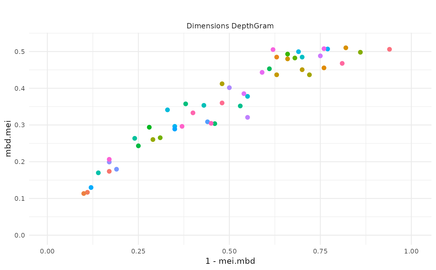
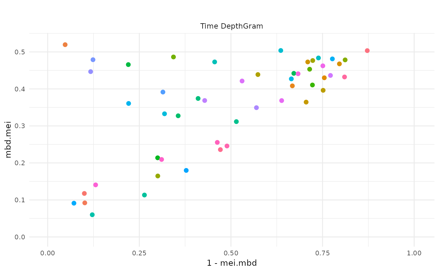
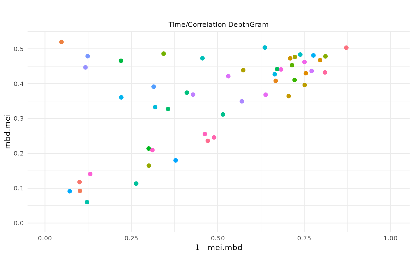
Specialized method to plot 'depthgram' objects

This function plots the three 'DepthGram' representations from the output of the depthgram function.

# S3 method for depthgram
plot(
  x,
  limits = FALSE,
  ids = NULL,
  print = FALSE,
  plot_title = "",
  shorten = TRUE,
  col = NULL,
  pch = 19,
  sp = 2,
  st = 4,
  sa = 10,
  text_labels = "",
  ...
)

Arguments

x: An object of class depthgram as output by the depthgram function.
limits: A boolean specifying whether the empirical limits for outlier detection should be drawn. Defaults to FALSE.
ids: A character vector specifying labels for individual observations. Defaults to NULL, in which case observations will named by their id number in order of appearance.
print: A boolean specifying whether the graphical output should be optimized for printed version. Defaults to FALSE.
plot_title: A character string specifying the main title for the plot. Defaults to "", which means no title.
shorten: A boolean specifying whether labels must be shorten to 15 characters. Defaults to TRUE.
col: Color palette used for the plot. Defaults to NULL, in which case a default palette produced by the hcl function is used.
pch: Point shape. See plotly for more details. Defaults to 19.
sp: Point size. See plotly for more details. Defaults to 2.
st: Label size. See plotly for more details. Defaults to 4.
sa: Axis title sizes. See plotly for more details. Defaults to 10.
text_labels: A character vector specifying the labels for the individuals. It is overridden if limits = TRUE, for which only outliers labels are shown. See plotly for more details. Defaults to "".
...: Other arguments to be passed to the base plot function. Unused.

Value

A list with the following items:

p: list with all the interactive (plotly) depthGram plots;
out: outliers detected;
colors: used colors for plotting.

References

Aleman-Gomez, Y., Arribas-Gil, A., Desco, M. Elias-Fernandez, A., and Romo, J. (2021). "Depthgram: Visualizing Outliers in High Dimensional Functional Data with application to Task fMRI data exploration".

Examples

N <- 50
P <- 50
grid <- seq(0, 1, length.out = P)
Cov <- exp_cov_function(grid, alpha = 0.3, beta = 0.4)

Data <- list()
Data[[1]] <- generate_gauss_fdata(
  N,
  centerline = sin(2 * pi * grid),
  Cov = Cov
)
Data[[2]] <- generate_gauss_fdata(
  N,
  centerline = sin(2 * pi * grid),
  Cov = Cov
)
names <- paste0("id_", 1:nrow(Data[[1]]))
DG <- depthgram(Data, marginal_outliers = TRUE, ids = names)
plot(DG)
#> $p
#> $p$dimDG

#> 
#> $p$timeDG

#> 
#> $p$corrDG

#> 
#> $p$fullDG
#> 
#> 
#> $out
#> NULL
#> 
#> $color
#>  [1] "#F8766D" "#F37B59" "#ED8141" "#E7861B" "#E08B00" "#D89000" "#CF9400"
#>  [8] "#C59900" "#BB9D00" "#AFA100" "#A3A500" "#95A900" "#85AD00" "#72B000"
#> [15] "#5BB300" "#39B600" "#00B81F" "#00BA42" "#00BC59" "#00BE6C" "#00BF7D"
#> [22] "#00C08D" "#00C19C" "#00C1AA" "#00C0B8" "#00BFC4" "#00BDD0" "#00BBDB"
#> [29] "#00B8E5" "#00B4EF" "#00B0F6" "#00ABFD" "#00A5FF" "#529EFF" "#7997FF"
#> [36] "#9590FF" "#AC88FF" "#BF80FF" "#CF78FF" "#DC71FA" "#E76BF3" "#F066EA"
#> [43] "#F763E0" "#FC61D5" "#FF61C9" "#FF62BC" "#FF65AE" "#FF689F" "#FF6C90"
#> [50] "#FC717F"
#>