
# A tibble: 5 × 4
  species flipper_length_mm body_mass_g   bmi
  <chr>               <dbl>       <dbl> <dbl>
1 Adelie                181        3750 1145.
2 Adelie                186        3800 1098.
3 Adelie                195        3250  855.
4 Adelie                 NA          NA   NA
5 Adelie 193 3450 926.Explore your data: the tidyverse
The R Statistical Language · Session 2
3.1 Why plot?
A plot is the fastest way to feel your data. Anscombe’s quartet is the classic proof: four data sets with nearly identical means, variances and correlations, yet plots that look nothing alike.
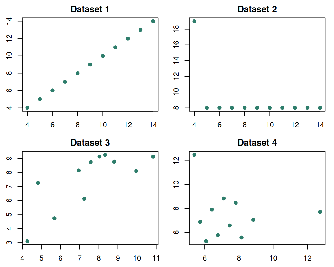
The four data sets share the same slope, intercept, correlation and means; only the plots tell them apart. A table could not, a hist() of a single column would not, an illustration does.
The lesson. Look at your data before you summarise it: a single well-chosen plot often tells you more than ten summary statistics. This is the heart of Exploratory Data Analysis.
## Why plot? {.inv}

A plot is the fastest way to *feel* your data. Anscombe's quartet is the classic proof: four data sets with nearly identical means, variances and correlations, yet plots that look nothing alike.

::: {.split-2}
```{r}
#| label: anscombe
#| echo: false
#| fig-width: 6
#| fig-height: 4.8
par(bg = "white")                 # opaque white figure so the black ink shows on the dark slide
par(mfrow = c(2, 2), mar = c(2.5, 2.5, 2, 1), cex = 0.8)
for (i in 1:4) {
  plot(anscombe[, c(2*i - 1, 2*i)], pch = 19, col = "#2E7D6B",
       main = paste0("Dataset ", i))
}
```

The four data sets share the same slope, intercept, correlation and means; only the *plots* tell them apart. A table could not, a `hist()` of a single column would not, an illustration does.

::: {.callout-desc}
**The lesson.** Look at your data before you summarise it: a single well-chosen plot often tells you more than ten summary statistics. This is the heart of *Exploratory Data Analysis*.
:::
:::
3.2 Histograms in base R
The simplest first look at one variable: hist().
hist.R
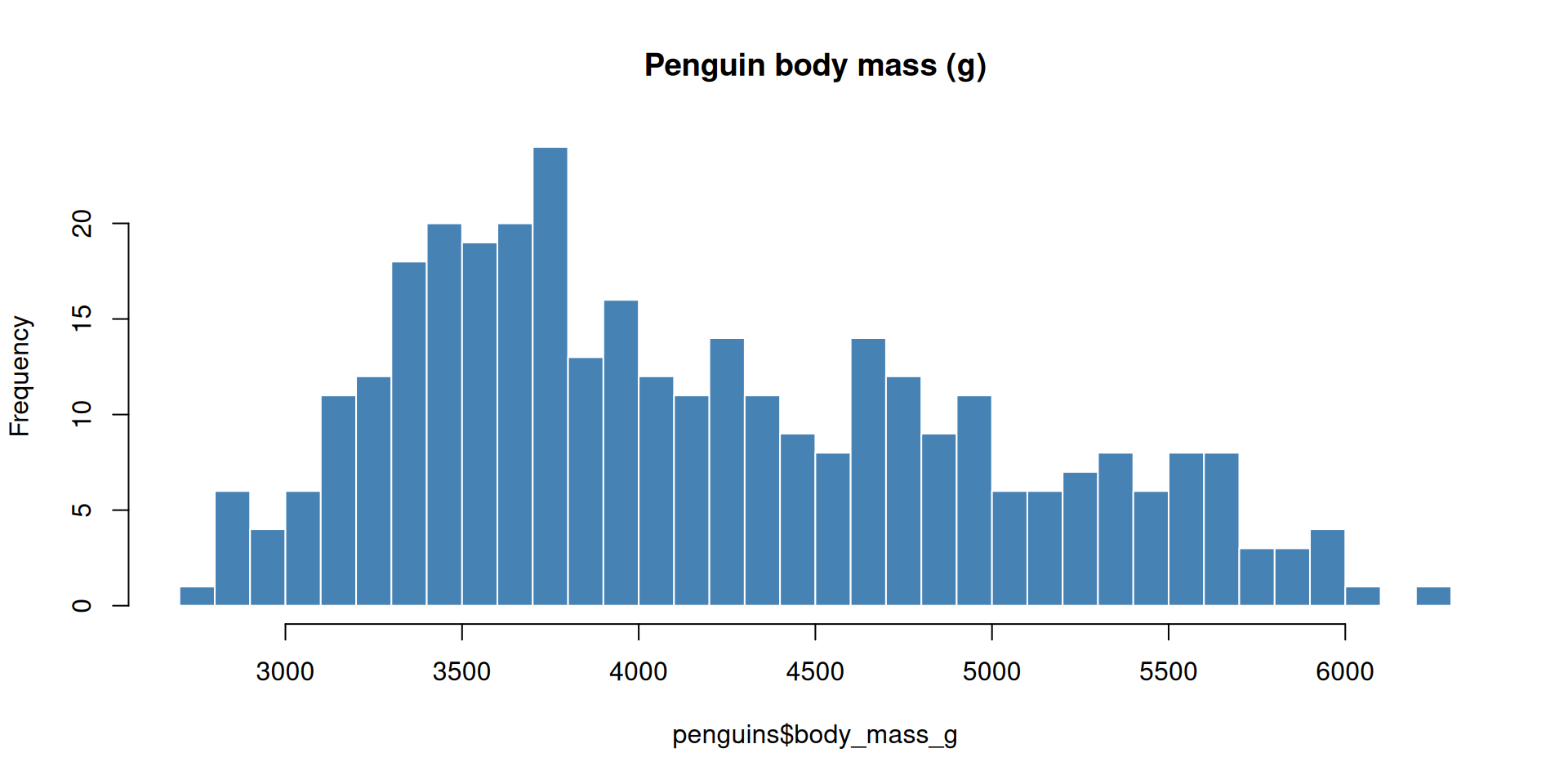
Positron draws the plot in the Plots pane. hist() is one call, but its defaults are utilitarian.
## Histograms in base R {.inv}
The simplest first look at one variable: **`hist()`**.
::: {.codewindow .r width="100%"}
hist.R
```{r}
#| echo: true
#| output-location: column
par(bg = "white")                # opaque white figure: dark slide would hide the default black ink
hist(
  penguins$body_mass_g,          # the variable
  breaks = 30,                   # how many bins
  col = "steelblue",
  border = "white",
  main = "Penguin body mass (g)" # title
)
```
:::
::: {.paper-card}
Positron draws the plot in the **Plots** pane. `hist()` is one call, but its defaults are utilitarian.
:::
3.3 Other base-R workhorses
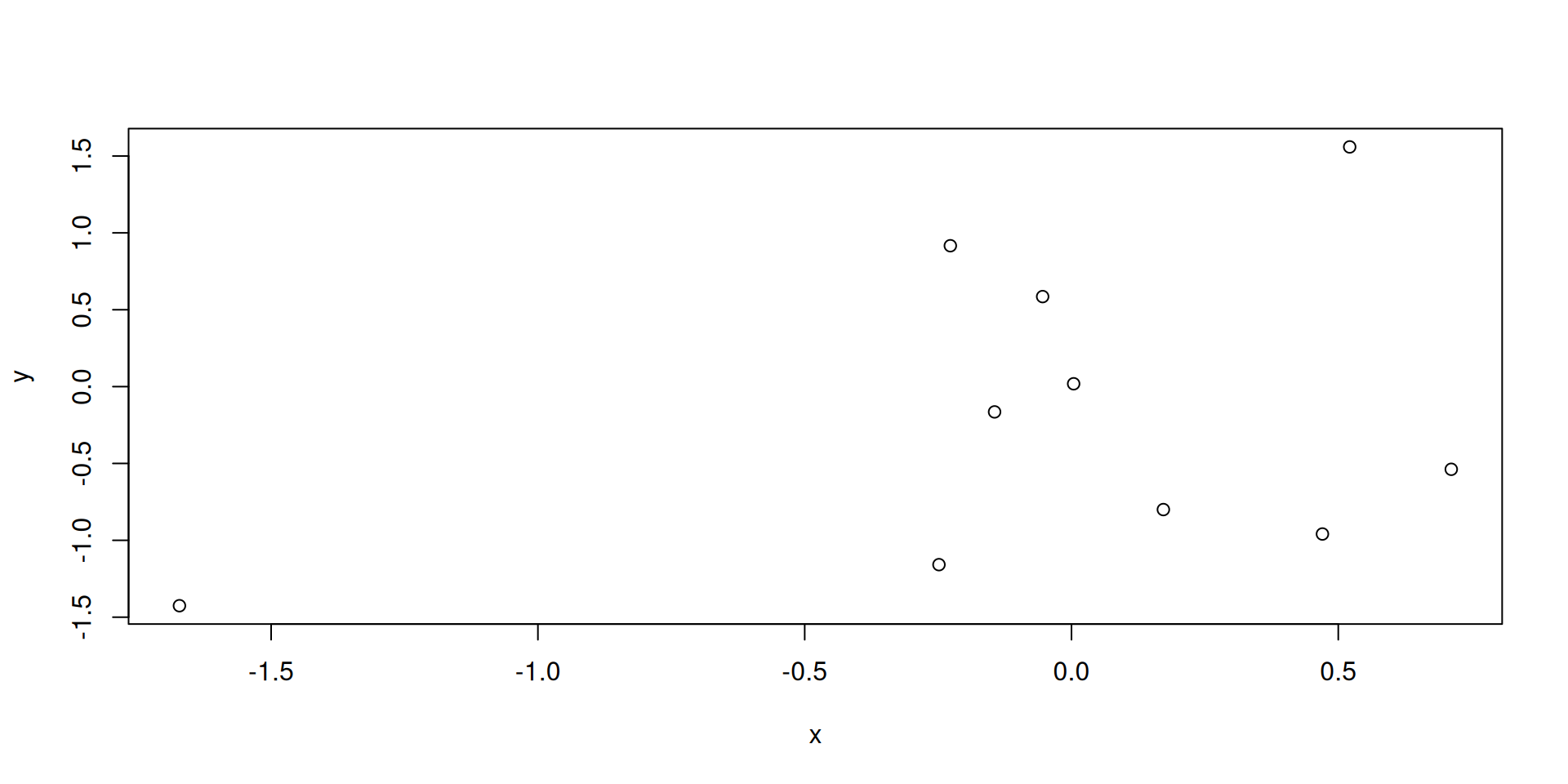
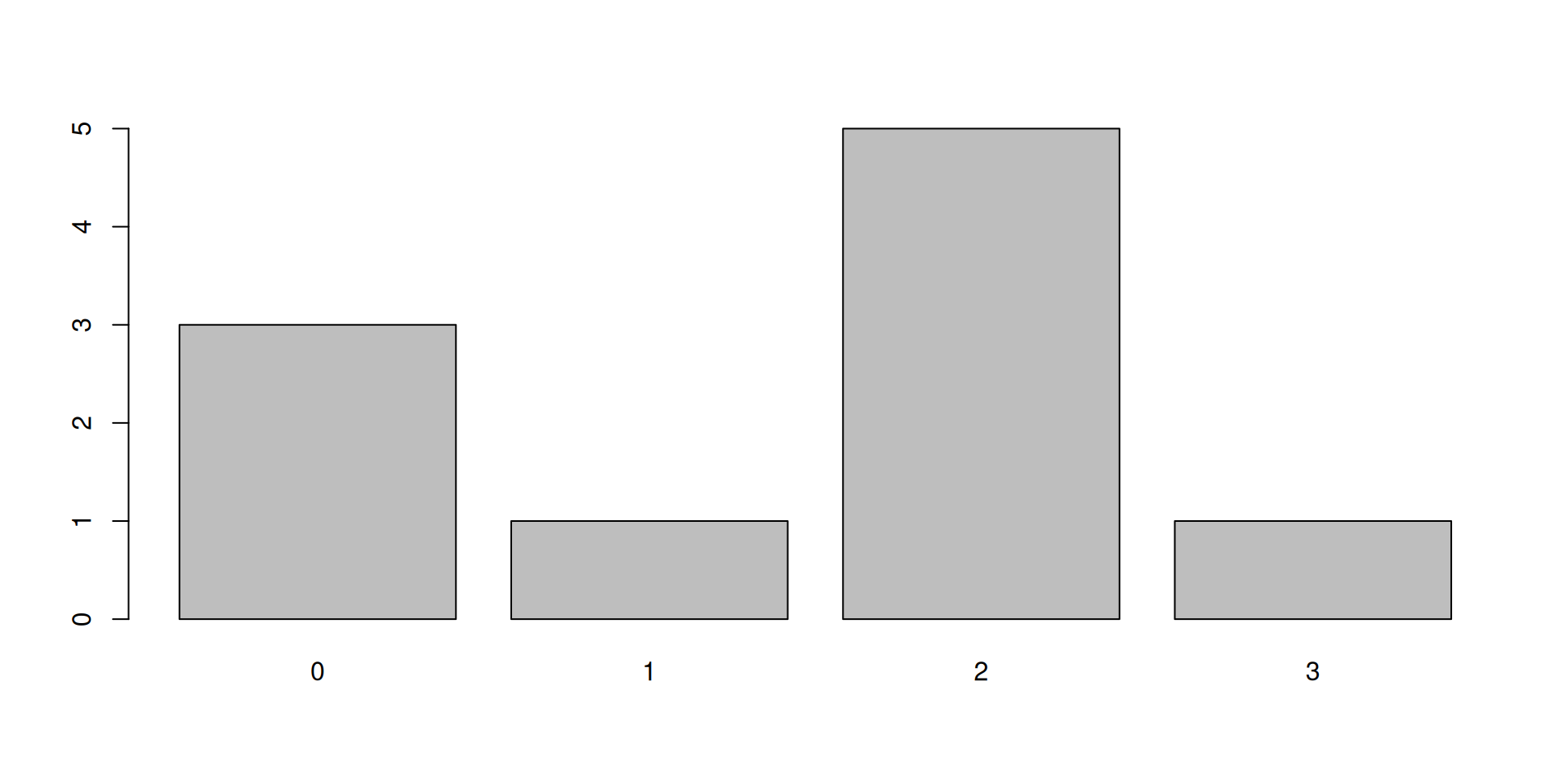
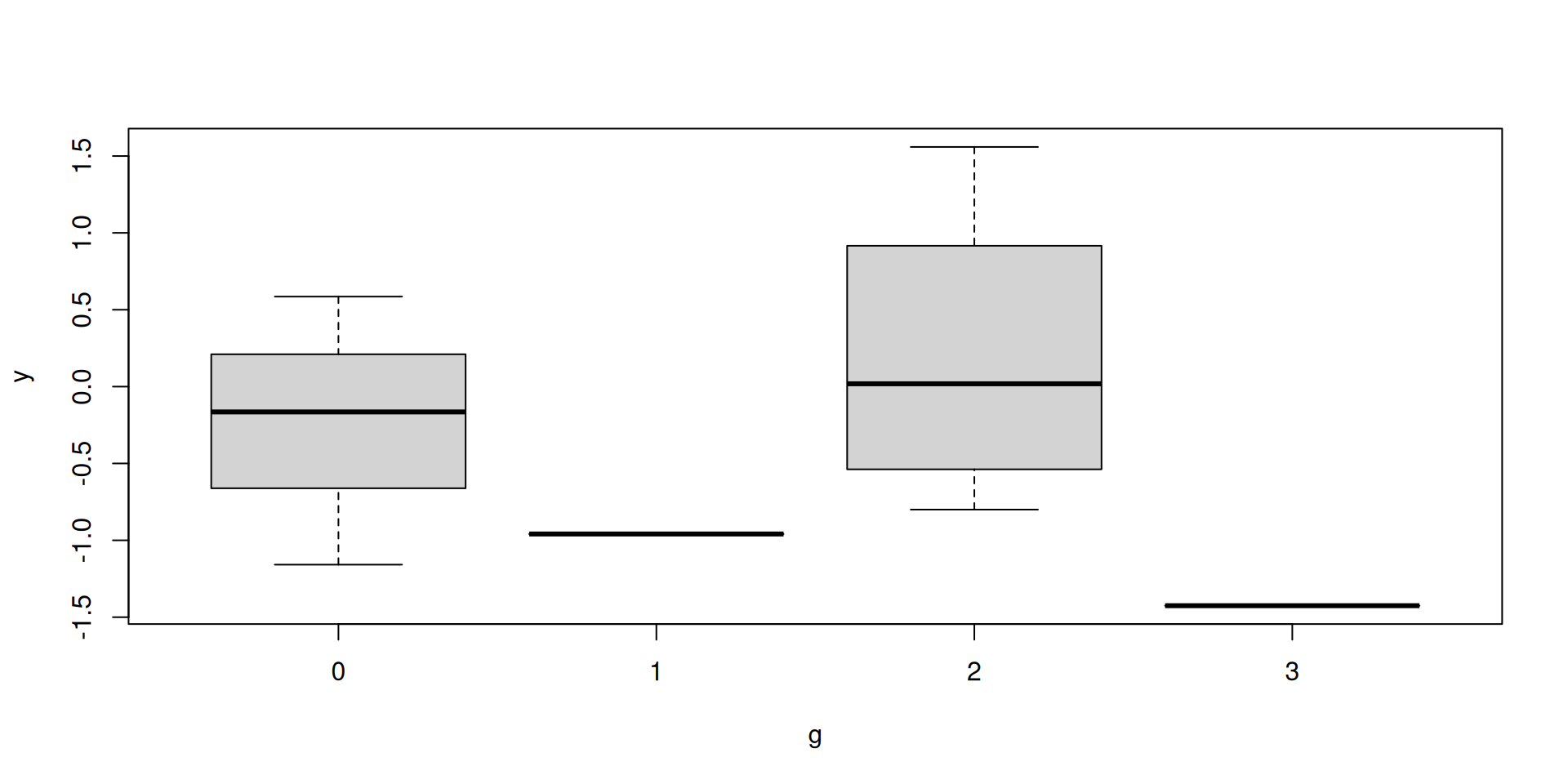
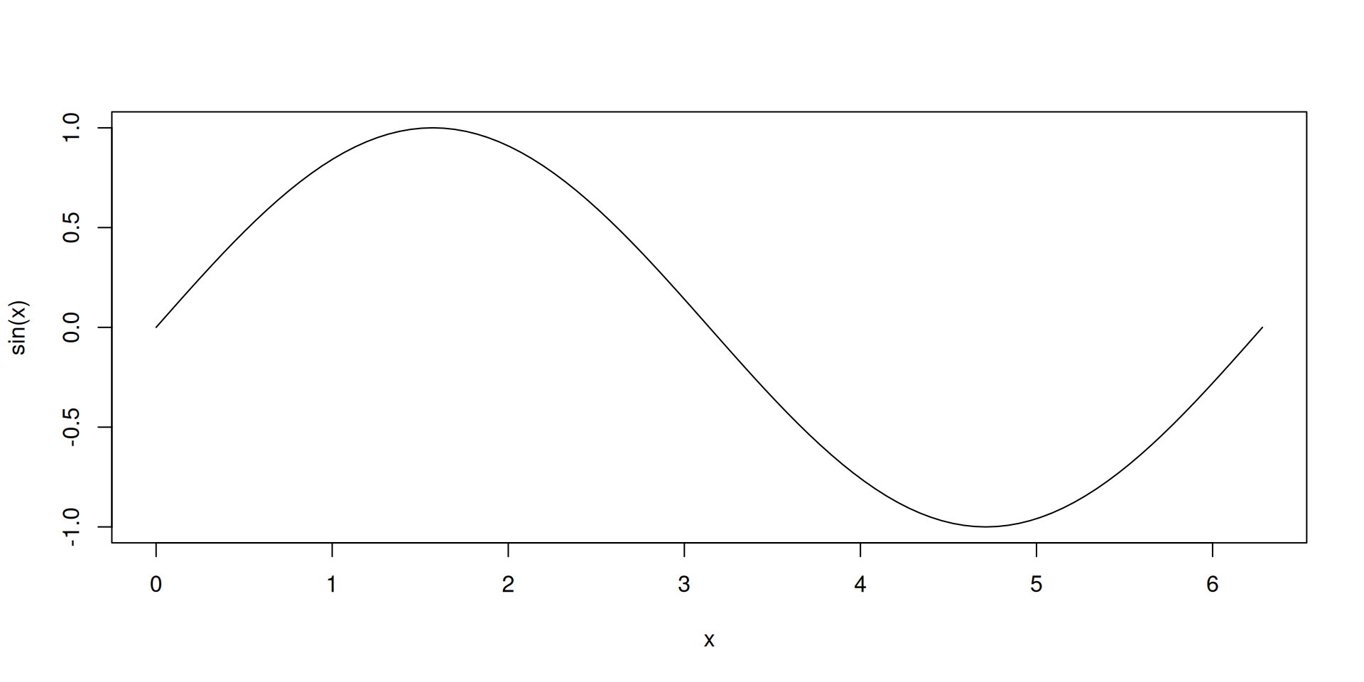
Base R can already do a lot, but its look is dated and customisation is verbose: why we meet ggplot2 next.
## Other base-R workhorses {.inv}
::: {.panel-tabset}
### Scatterplot
::: {.codewindow .r width="100%"}
The rest of the base-R drawer
```{r}
#| echo: true
#| output-location: column
par(bg = "white")   # opaque white figure so the default black ink shows on the dark slide
x <- rnorm(10)
y <- rnorm(10)
plot(x, y)          # scatter plot
```
:::
### Barplot
::: {.codewindow .r width="100%"}
The rest of the base-R drawer
```{r}
#| echo: true
#| output-location: column
par(bg = "white")   # opaque white figure so the default black ink shows on the dark slide
g <- rpois(n = 10L, lambda = 1)
barplot(table(g))   # counts of categories
```
:::
### Boxplot
::: {.codewindow .r width="100%"}
The rest of the base-R drawer
```{r}
#| echo: true
#| output-location: column
par(bg = "white")   # opaque white figure so the default black ink shows on the dark slide
boxplot(y ~ g)      # one box per group
```
:::
### Function plotting
::: {.codewindow .r width="100%"}
The rest of the base-R drawer
```{r}
#| echo: true
#| output-location: column
par(bg = "white")   # opaque white figure so the default black ink shows on the dark slide
curve(sin, 0, 2*pi) # plot a function
```
:::
:::
::: {.paper-card}
Base R can already do a lot, but its look is dated and customisation is verbose: *why* we meet **ggplot2** next.
:::
4.2 The first ggplot
Every plot starts with ggplot(data = , mapping = aes(...)), then adds layers with +:
ggplot(
    data = penguins,
    mapping = aes(x = body_mass_g)
  ) +
geom_histogram(bins = 30, color = "white")
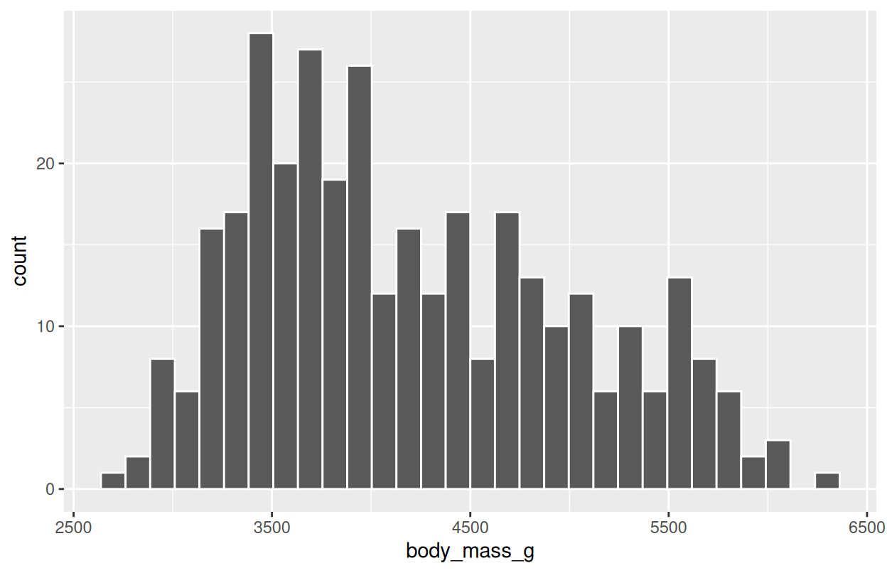
This is the same histogram we drew in base R, but now each piece is explicit and easy to extend.
## The first ggplot {.inv}

Every plot starts with `ggplot(data = , mapping = aes(...))`, then adds layers with `+`:

::: {.split-2}
<div class="code-build">
  <pre class="fragment" data-fragment-index="1">ggplot(
    data = penguins,
    mapping = aes(x = body_mass_g)
  ) + </pre>
  <pre class="fragment cb-cur" data-fragment-index="2">  geom_histogram(bins = 30, color = "white")</pre>
</div>

::: {.plot-stack}
```{r}
#| echo: false
#| fig-width: 6.5
#| fig-height: 4.2
#| out.extra: 'class="fragment step-plot" data-fragment-index="1"'
ggplot(
  data = penguins,
  mapping = aes(x = body_mass_g)
)
```

```{r}
#| echo: false
#| fig-width: 6.5
#| fig-height: 4.2
#| out.extra: 'class="fragment step-plot" data-fragment-index="2"'
ggplot(
  data = penguins,
  mapping = aes(x = body_mass_g)
) +
  geom_histogram(bins = 30, color = "white")
```
:::
:::

::: {.paper-card .fragment}
This is the *same histogram* we drew in base R, but now each piece is explicit and easy to extend.
:::
4.3 Scatter: two continuous variables
Mapping variables to x and y, and a third to color:
ggplot(
    data = penguins,
    mapping = aes(x = flipper_length_mm, y = body_mass_g)
  ) +
geom_point(aes(color = species), alpha = 0.7) +
theme_dark() +
  labs(
    title = "Body mass variation with flipper length",
    caption = "Data from the {palmerpengins} package.",
    x = "Flipper Length (mm)",
    y = "Body Mass (g)",
    color = "Species"
  )
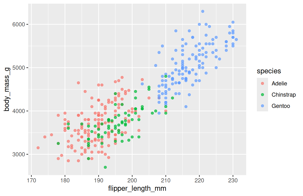
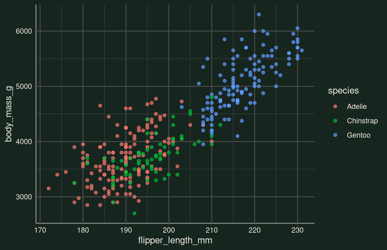
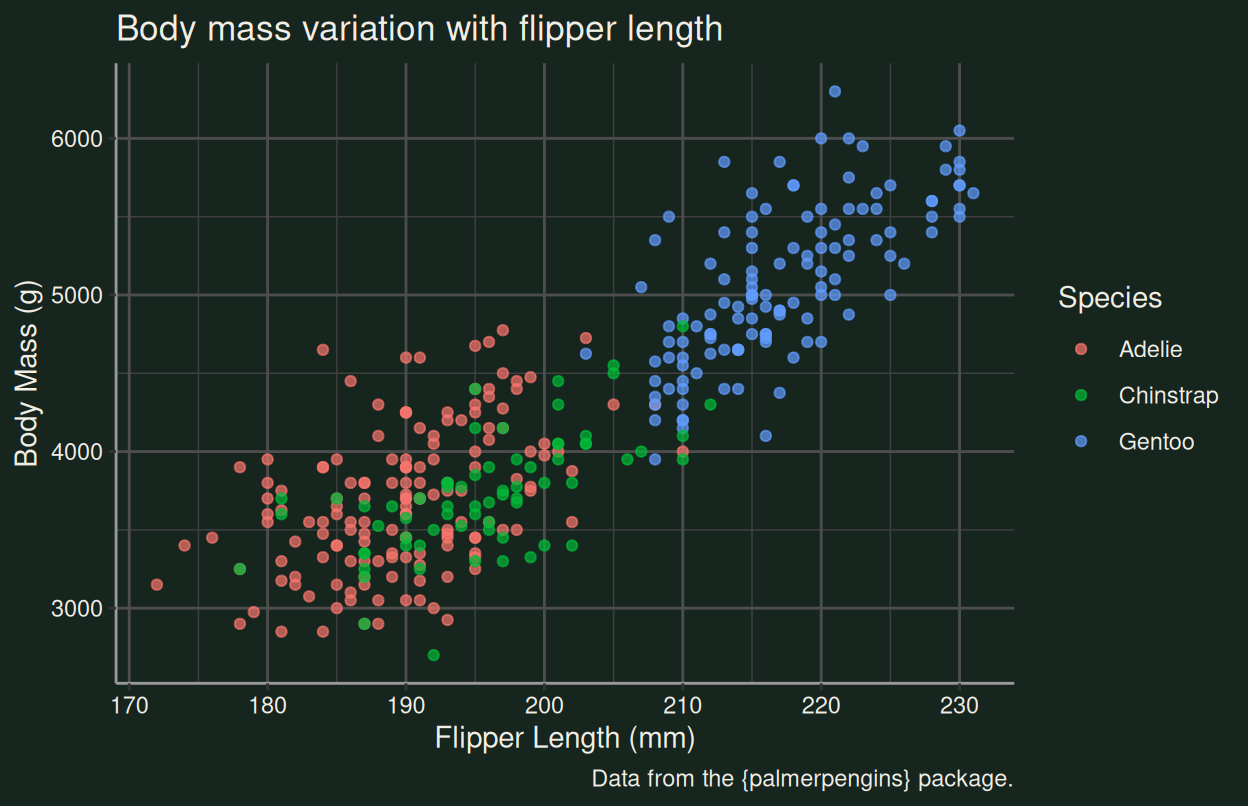
Read it aloud. “Body mass grows with flipper length”, and each species clusters in its own region of this space. That’s a finding you’d never see from summary().
## Scatter: two continuous variables {.inv}

Mapping variables to `x` and `y`, and a third to `color`:

::: {.split-2}
<div class="code-build">
  <pre class="fragment" data-fragment-index="1">ggplot(
    data = penguins,
    mapping = aes(x = flipper_length_mm, y = body_mass_g)
  ) + </pre>
  <pre class="fragment cb-cur" data-fragment-index="2">  geom_point(aes(color = species), alpha = 0.7) + </pre>
  <pre class="fragment cb-cur" data-fragment-index="3">  theme_dark() + </pre>
  <pre class="fragment cb-cur" data-fragment-index="4">  labs(
    title = "Body mass variation with flipper length",
    caption = "Data from the {palmerpengins} package.",
    x = "Flipper Length (mm)",
    y = "Body Mass (g)",
    color = "Species"
  )</pre>
</div>

::: {.plot-stack}
```{r}
#| echo: false
#| fig-width: 6.5
#| fig-height: 4.2
#| out.extra: 'class="fragment step-plot" data-fragment-index="1"'
ggplot(penguins, aes(x = flipper_length_mm, y = body_mass_g))
```

```{r}
#| echo: false
#| fig-width: 6.5
#| fig-height: 4.2
#| out.extra: 'class="fragment step-plot" data-fragment-index="2"'
ggplot(penguins, aes(x = flipper_length_mm, y = body_mass_g)) +
  geom_point(aes(color = species), alpha = 0.7)
```

```{r}
#| echo: false
#| fig-width: 6.5
#| fig-height: 4.2
#| out.extra: 'class="fragment step-plot" data-fragment-index="3"'
ggplot(penguins, aes(x = flipper_length_mm, y = body_mass_g)) +
  geom_point(aes(color = species), alpha = 0.7) +
  theme_dark()
```

```{r}
#| echo: false
#| fig-width: 6.5
#| fig-height: 4.2
#| out.extra: 'class="fragment step-plot" data-fragment-index="4"'
ggplot(penguins, aes(x = flipper_length_mm, y = body_mass_g)) +
  geom_point(aes(color = species), alpha = 0.7) +
  theme_dark() +
  labs(
    title = "Body mass variation with flipper length",
    caption = "Data from the {palmerpengins} package.",
    x = "Flipper Length (mm)",
    y = "Body Mass (g)",
    color = "Species"
  )
```
:::
:::

::: {.paper-card .fragment}
**Read it aloud.** "Body mass grows with flipper length", and each species clusters in its own region of this space. That's a finding you'd never see from `summary()`.
:::
4.4 One variable per facet
Faceting splits the plot into small multiples: one per level of a variable:
ggplot(
    data = penguins,
    mapping = aes(x = body_mass_g)
  ) +
  geom_histogram(
    bins = 25,
    fill = "#2E7D6B",
    color = "#17251F"
  ) +
  facet_wrap(
    facets = vars(species),
    ncol = 1
  ) +
theme_dark()
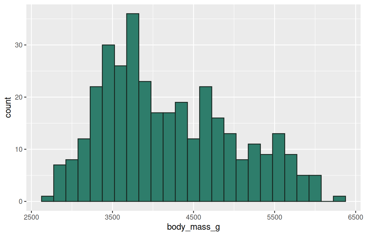
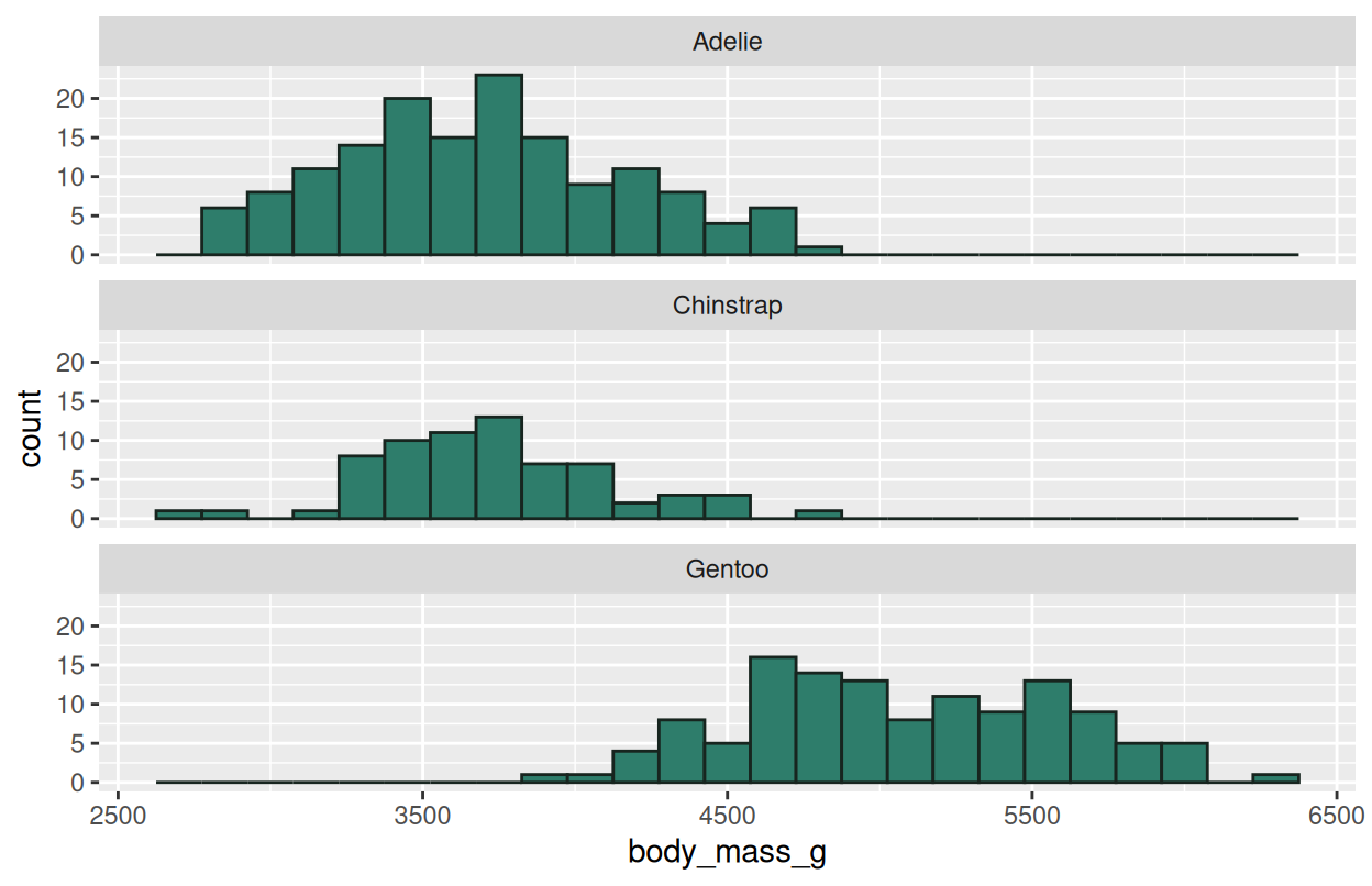
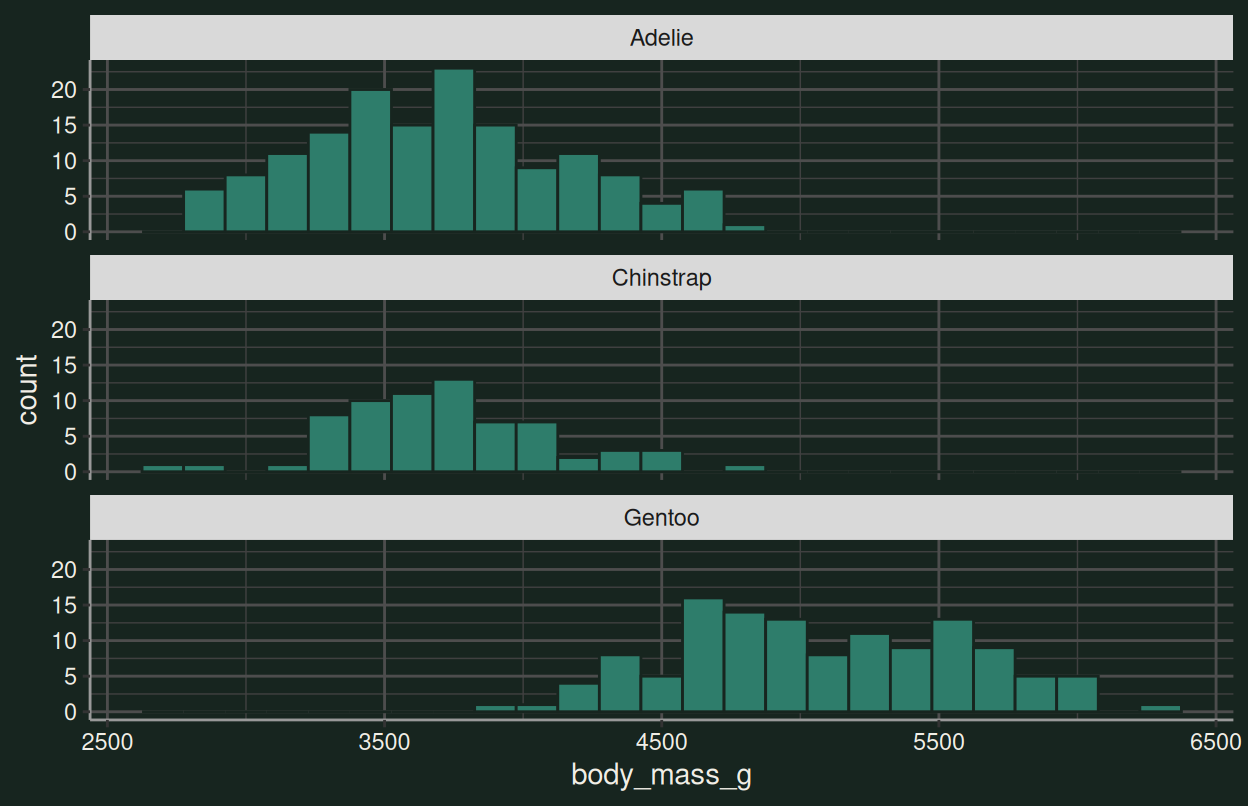
Different species have different distributions of body mass: a comparison that’s hard to see in one pooled histogram.
## One variable per facet {.inv}

**Faceting** splits the plot into small multiples: one per level of a variable:

::: {.split-2}
<div class="code-build">
  <pre class="fragment" data-fragment-index="1">ggplot(
    data = penguins,
    mapping = aes(x = body_mass_g)
  ) + </pre>
  <pre class="fragment cb-cur" data-fragment-index="2">  geom_histogram(
    bins = 25,
    fill = "#2E7D6B",
    color = "#17251F"
  ) + </pre>
  <pre class="fragment cb-cur" data-fragment-index="3">  facet_wrap(
    facets = vars(species),
    ncol = 1
  ) + </pre>
  <pre class="fragment cb-cur" data-fragment-index="4">  theme_dark()</pre>
</div>

::: {.plot-stack}
```{r}
#| echo: false
#| fig-width: 6.5
#| fig-height: 4.2
#| out.extra: 'class="fragment step-plot" data-fragment-index="1"'
ggplot(penguins, aes(x = body_mass_g))
```

```{r}
#| echo: false
#| fig-width: 6.5
#| fig-height: 4.2
#| out.extra: 'class="fragment step-plot" data-fragment-index="2"'
ggplot(penguins, aes(x = body_mass_g)) +
  geom_histogram(bins = 25, fill = "#2E7D6B", color = "#17251F")
```

```{r}
#| echo: false
#| fig-width: 6.5
#| fig-height: 4.2
#| out.extra: 'class="fragment step-plot" data-fragment-index="3"'
ggplot(penguins, aes(x = body_mass_g)) +
  geom_histogram(bins = 25, fill = "#2E7D6B", color = "#17251F") +
  facet_wrap(~ species, ncol = 1)
```

```{r}
#| echo: false
#| fig-width: 6.5
#| fig-height: 4.2
#| out.extra: 'class="fragment step-plot" data-fragment-index="4"'
ggplot(penguins, aes(x = body_mass_g)) +
  geom_histogram(bins = 25, fill = "#2E7D6B", color = "#17251F") +
  facet_wrap(~ species, ncol = 1) +
  theme_dark()
```
:::
:::

::: {.paper-card .fragment}
Different species have *different* distributions of body mass: a comparison that's hard to see in one pooled histogram.
:::
4.5 Boxplots for groups
Categorical x + continuous y:
ggplot(
    data = penguins,
    mapping = aes(x = species, y = bill_length_mm, fill = species)
  ) +
geom_boxplot(alpha = 0.8) +
theme_dark() +
theme(legend.position = "none")
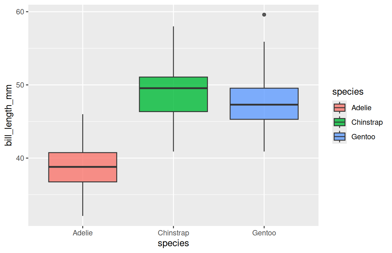
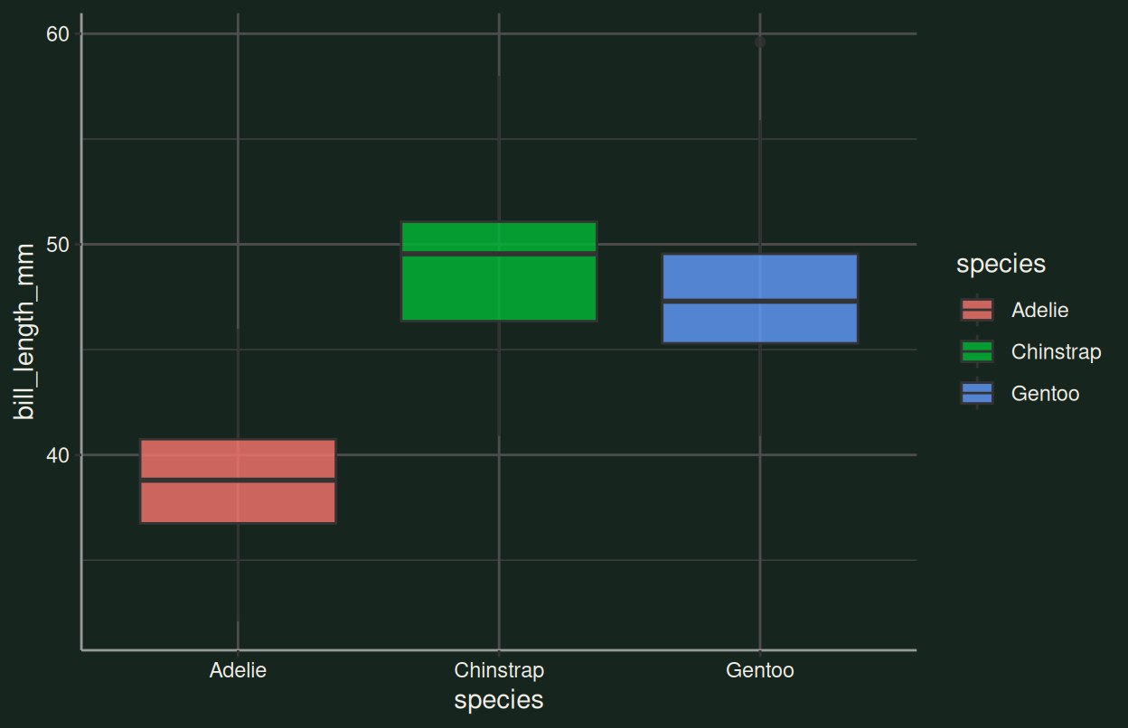
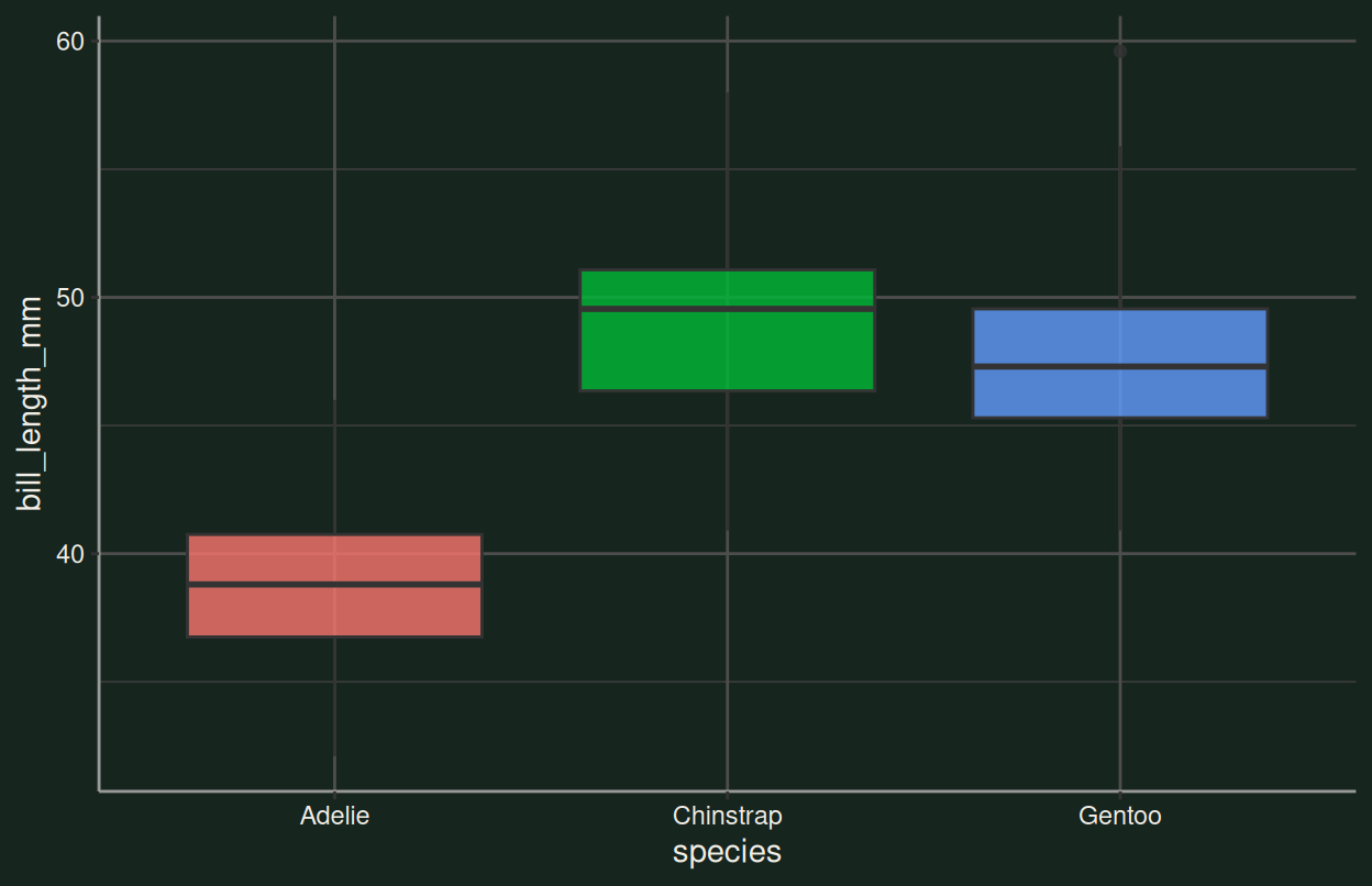
A boxplot shows the median, the box (IQR) and outliers at a glance: ideal for comparing a numeric variable across groups.
## Boxplots for groups {.inv}

Categorical `x` + continuous `y`:

::: {.split-2}
<div class="code-build">
  <pre class="fragment" data-fragment-index="1">ggplot(
    data = penguins,
    mapping = aes(x = species, y = bill_length_mm, fill = species)
  ) + </pre>
  <pre class="fragment cb-cur" data-fragment-index="2">  geom_boxplot(alpha = 0.8) + </pre>
  <pre class="fragment cb-cur" data-fragment-index="3">  theme_dark() + </pre>
  <pre class="fragment cb-cur" data-fragment-index="4">  theme(legend.position = "none")</pre>
</div>

::: {.plot-stack}
```{r}
#| echo: false
#| fig-width: 6.5
#| fig-height: 4.2
#| out.extra: 'class="fragment step-plot" data-fragment-index="1"'
ggplot(penguins, aes(x = species, y = bill_length_mm, fill = species))
```

```{r}
#| echo: false
#| fig-width: 6.5
#| fig-height: 4.2
#| out.extra: 'class="fragment step-plot" data-fragment-index="2"'
ggplot(penguins, aes(x = species, y = bill_length_mm, fill = species)) +
  geom_boxplot(alpha = 0.8)
```

```{r}
#| echo: false
#| fig-width: 6.5
#| fig-height: 4.2
#| out.extra: 'class="fragment step-plot" data-fragment-index="3"'
ggplot(penguins, aes(x = species, y = bill_length_mm, fill = species)) +
  geom_boxplot(alpha = 0.8) +
  theme_dark()
```

```{r}
#| echo: false
#| fig-width: 6.5
#| fig-height: 4.2
#| out.extra: 'class="fragment step-plot" data-fragment-index="4"'
ggplot(penguins, aes(x = species, y = bill_length_mm, fill = species)) +
  geom_boxplot(alpha = 0.8) +
  theme_dark() +
  theme(legend.position = "none")
```
:::
:::

::: {.paper-card .fragment}
A boxplot shows the median, the box (IQR) and outliers at a glance: ideal for comparing a numeric variable *across groups*.
:::
4.6 Order factors with {forcats}
{forcats} lets you reorder those levels so graphs tell the story you want:
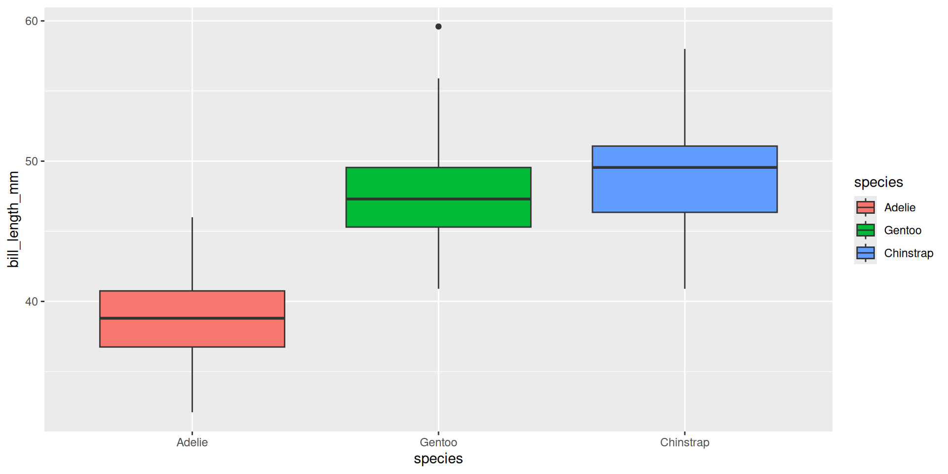
fct_reorder() puts the highest median first on the axis: order becomes part of your message. fct_relevel/fct_lump fine-tune and collapse rare levels.
## Order factors with [{forcats}](https://forcats.tidyverse.org) {.inv}
[{forcats}](https://forcats.tidyverse.org) lets you **reorder** those levels so graphs tell the story you want:
::: {.codewindow .r width="100%" name="fct-reorder.R"}
```{r}
#| echo: true
#| output-location: column
penguins |>
  dplyr::mutate(species = forcats::fct_reorder(
    .f = species,
    .x = bill_length_mm,
    .fun = median,
    na.rm = TRUE
  )) |>
  ggplot(mapping = aes(
    x = species,
    y = bill_length_mm,
    fill = species
  )) +
  geom_boxplot()
```
:::
::: {.paper-card}
`fct_reorder()` puts the *highest median first* on the axis: order becomes part of your message. `fct_relevel`/`fct_lump` fine-tune and collapse rare levels.
:::
4.7 Layers compose
An important ggplot2 habit: plots are built from many layers. For example, scatter + a smooth trend:
ggplot(
    data = penguins,
    mapping = aes(x = flipper_length_mm, y = body_mass_g)
  ) +
geom_point(aes(color = species), alpha = 0.6) +
  geom_smooth(
    method = "lm",
    se = FALSE,
    color = "#E8A33D",
    linewidth = 1
  ) +
theme_dark()
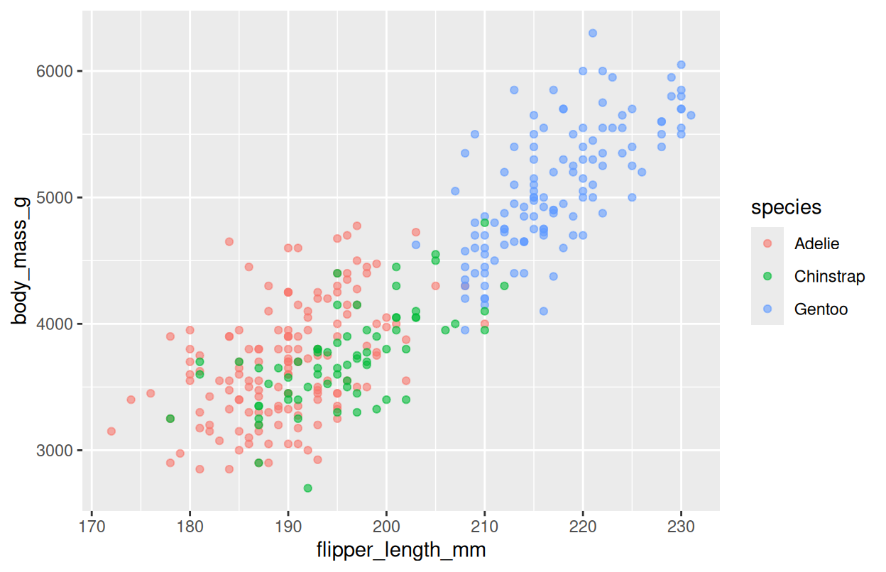
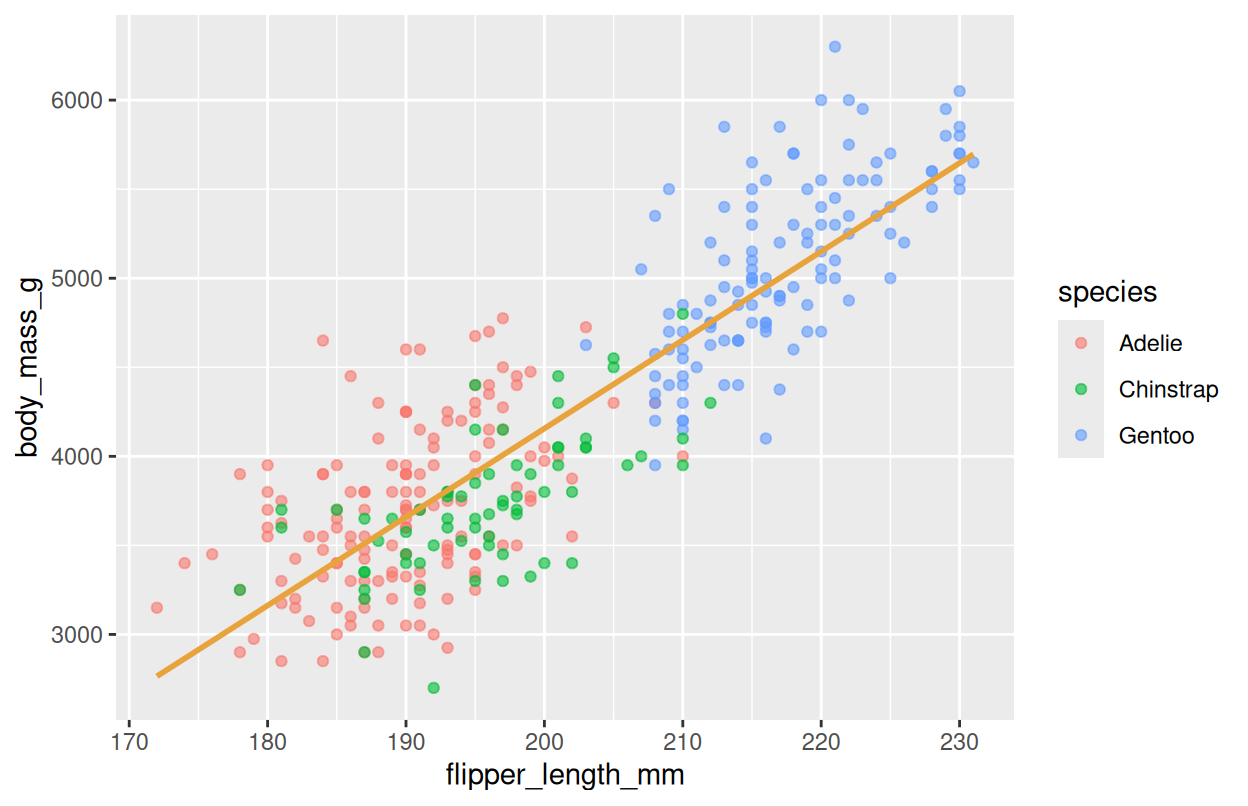
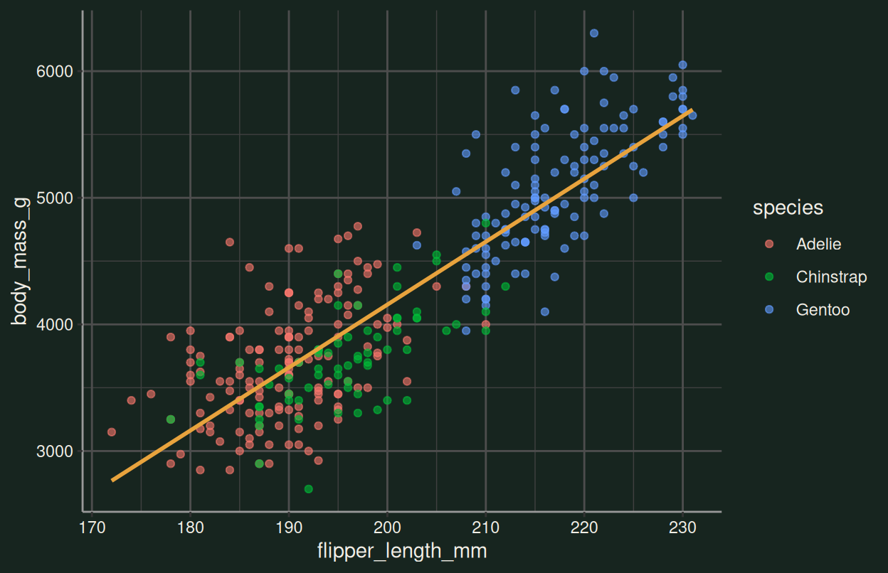
geom_point() and geom_smooth() layer on the same plot, each with its own mapping. This layering is what makes ggplot2 so expressive.
## Layers compose {.inv}

An important ggplot2 habit: plots are built from **many layers**. For example, scatter + a smooth trend:

::: {.split-2}
<div class="code-build">
  <pre class="fragment" data-fragment-index="1">ggplot(
    data = penguins,
    mapping = aes(x = flipper_length_mm, y = body_mass_g)
  ) + </pre>
  <pre class="fragment cb-cur" data-fragment-index="2">  geom_point(aes(color = species), alpha = 0.6) + </pre>
  <pre class="fragment cb-cur" data-fragment-index="3">  geom_smooth(
    method = "lm",
    se = FALSE,
    color = "#E8A33D",
    linewidth = 1
  ) + </pre>
  <pre class="fragment cb-cur" data-fragment-index="4">  theme_dark()</pre>
</div>

::: {.plot-stack}
```{r}
#| echo: false
#| fig-width: 6.5
#| fig-height: 4.2
#| out.extra: 'class="fragment step-plot" data-fragment-index="1"'
ggplot(penguins, aes(x = flipper_length_mm, y = body_mass_g))
```

```{r}
#| echo: false
#| fig-width: 6.5
#| fig-height: 4.2
#| out.extra: 'class="fragment step-plot" data-fragment-index="2"'
ggplot(penguins, aes(x = flipper_length_mm, y = body_mass_g)) +
  geom_point(aes(color = species), alpha = 0.6)
```

```{r}
#| echo: false
#| fig-width: 6.5
#| fig-height: 4.2
#| out.extra: 'class="fragment step-plot" data-fragment-index="3"'
ggplot(penguins, aes(x = flipper_length_mm, y = body_mass_g)) +
  geom_point(aes(color = species), alpha = 0.6) +
  geom_smooth(method = "lm", se = FALSE, color = "#E8A33D", linewidth = 1)
```

```{r}
#| echo: false
#| fig-width: 6.5
#| fig-height: 4.2
#| out.extra: 'class="fragment step-plot" data-fragment-index="4"'
ggplot(penguins, aes(x = flipper_length_mm, y = body_mass_g)) +
  geom_point(aes(color = species), alpha = 0.6) +
  geom_smooth(method = "lm", se = FALSE, color = "#E8A33D", linewidth = 1) +
  theme_dark()
```
:::
:::

::: {.paper-card .fragment}
`geom_point()` and `geom_smooth()` *layer* on the same plot, each with its own mapping. This layering is what makes ggplot2 so expressive.
:::
