The tractoverse

White matter tractography analysis in R

Aymeric Stamm

Department of Mathematics Jean Leray, UMR CNRS 6629, Nantes, France

July 9, 2026

The brain’s white matter

Diffusion MRI probes water motion in tissue at the micron scale.

• Axons restrict diffusion along their axis → anisotropy
• Magnetic field gradient attenuates the MR signal → diffusion-weighted images
• Voxel-level diffusion model → local fiber orientation and tissue properties

Tractography follows these orientations across voxels to reconstruct 3-D fiber trajectories which carry microstructural information.

Taken from Wikimedia Commons - under CC BY 3.0 license

%%{init:{"theme":"dark","themeVariables":{"fontSize":"16px"}}}%%
flowchart TD
  A["🧠 Diffusion MRI<br/>(raw signal)"]:::blue --> B["Preprocessing<br/>(Eddy, motion, B0)"]:::grey
  B --> C["Diffusion model<br/>(DTI, CSD, NODDI…)"]:::blue
  C --> D["Tractography algorithm<br/>(deterministic / probabilistic)"]:::blue
  D --> E["🔗 Streamlines<br/>(ordered 3-D points)"]:::green
  E --> F1["Tractometry<br/>(microstructure along tract)"]:::teal
  E --> F2["Connectomics<br/>(region-to-region graph)"]:::teal
  E --> F3["Shape analysis<br/>(FDA, optimal transport)"]:::teal

  classDef blue fill:#1c3d5a,stroke:#58a6ff,color:#e6edf3
  classDef green fill:#1a3a2a,stroke:#3fb950,color:#e6edf3
  classDef teal fill:#1a3035,stroke:#39c5cf,color:#e6edf3
  classDef grey fill:#21262d,stroke:#8b949e,color:#8b949e

The R gap

Major tractography tools — none in R:

Software	Language	Analysis?
MRtrix3	C++	Connectomics
DIPY	Python	Connectomics + Tractometry
pyAFQ	Python	Tractometry
Scilpy	Python	Connectomics + Tractometry
DSI Studio	C++	Connectomics

(15+ tools surveyed — 0 in R)

R packages on CRAN for diffusion MRI:

dti — diffusion tensor fitting only, GPL, 47 dependencies

tractor.base — preprocessing pipeline, no streamline analysis

dmri.tracking — archived ✗

No R package provides comprehensively:

streamline objects tractometry connectomics shape analysis 3-D visualization microstructure simulation

The tractoverse

A modular collection of R packages for tractography analysis — inspired by the tidyverse.

Package	CRAN	Role
fiber	✅	Data structures
riot	⏳	I/O (awaiting rvtk)
rtists	🔜	3-D visualization
mascot	🔜	Reference datasets
midi	✅	Microstructure sim
bot	🔜	Optimal transport

+ rvtk — VTK infrastructure for R (v0.2.0 submitted)

Apr 2024midi 0.1.0first CRAN release

May 2026rvtk 0.1.3first CRAN release

Jun 2026fiber 0.1.0first CRAN release

Jul 2026fiber 0.2.0
midi 0.2.0latest updates

Jul 2026rvtk 0.2.0under submission

soon™riot
rtists
mascot
botpending / in development

fiber — S7 data structures

The backbone of the tractoverse. Like tibble is to the tidyverse. Three S7 classes:

streamline — one tract
@points (\(P \times 3\) matrix)
@point_data (list of length-\(P\) numeric vectors)
@streamline_data (list of scalars)

bundle — collection of streamlines
@streamlines (list of \(S\) streamlines)
@streamline_data (list of length-\(S\) numeric vectors)
@bundle_data (list of scalars)

bundle_set — multi-subject / multi-session
@bundles (list of \(B\) bundles)
@bundle_data (list of length-\(B\) numeric vectors)
@set_data (list of scalars)

Data lifting and subsetting
✅ @streamline_data common to all streamlines in a bundle → lifted to @streamline_data of the bundle;
✅ @bundle_data common to all bundles in a set → lifted to @set_data of the bundle set.
✅ Upon subsetting, lifted data is propagated down to the lower-level objects.

fiber — quick start

library(fiber)

t <- seq(0, 2 * pi, length.out = 50)

# Build a helix streamline
sl <- streamline(
  points     = cbind(X = cos(t), Y = sin(t), Z = t / (2 * pi)),
  point_data = list(FA = runif(50, 0.3, 0.9))
)
sl
#> ── Object of class `fiber::streamline()` with 50 points. ──
#>  • Point attributes: FA
#>  • Streamline attributes: none

# Geometry on streamlines
get_curvilinear_length(sl)   #> [1] 6.36
get_sinuosity(sl)            #> [1] 6.36

# Build a bundle and reparametrize
b <- bundle(lapply(1:10, \(i) reparametrize(sl, n_points = 20L)))
b
#> ── Object of class `fiber::bundle()` with 10 streamlines [20-20 pts/sl] ──

# Multi-subject bundle set
bs <- bundle_set(list("sub-01" = b, "sub-02" = b))
bs
#> ── Object of class `fiber::bundle_set()` with 2 bundles [10-10 sl/bundle] ──

✅ On CRAN  |  📦 Install: install.packages("fiber")  |  🔗 tractoverse.github.io/fiber

riot — R I/O for Tractography

Read & write tractography files in R — like readr is to the tidyverse.

Supported formats:

Format	Read	Write
VTK legacy .vtk	✅	✅
VTK XML .vtp	✅	✅
medInria .fds	✅	✅
MRtrix .tck/.tsf	✅	—
TrackVis .trk	✅	—
DIPY .dpy	✅	—

Returns fiber::streamline or fiber::bundle objects.

⏳ Not yet on CRAN — awaiting rvtk (v0.2.0) approval.

rvtk — VTK in R (not part of tractoverse)

%%{init:{"theme":"dark"}}%%
flowchart LR
  R["R package<br/>(riot)"] --> rvtk["rvtk<br/>(infrastructure)"]
  rvtk --> VTK["VTK C++ library<br/>(auto-downloaded)"]

  style R fill:#1c3d5a,stroke:#58a6ff,color:#e6edf3
  style rvtk fill:#2d1f52,stroke:#a371f7,color:#e6edf3
  style VTK fill:#1a3a2a,stroke:#3fb950,color:#e6edf3

• Searches for installed VTK or downloads prebuilt static libs
• No system dependency for end users
• use_rvtk() sets up any downstream package in one call
• Under CRAN submission as rvtk v0.2.0

🔗 astamm.github.io/rvtk

riot — reading any format

library(riot)

# VTK (all three sub-formats share the same read_bundle() API)
uf_vtk  <- read_bundle(system.file("extdata", "UF_left.vtk",  package = "riot"))
uf_vtp  <- read_bundle(system.file("extdata", "UF_left.vtp",  package = "riot"))
uf_fds  <- read_bundle(system.file("extdata", "UF_left.fds",  package = "riot"))

# MRtrix and TrackVis
af_tck  <- read_bundle(system.file("extdata", "AF_left.tck",  package = "riot"))
cc_trk  <- read_bundle(system.file("extdata", "CCMid.trk",    package = "riot"))

af_tck
#> <bundle [5000 streamlines | 8–54 pts/streamline]>

# Attach metadata at read time
uf_meta <- read_bundle(
  system.file("extdata", "UF_left.vtk", package = "riot"),
  bundle_data = list(subject = "sub-01", hemisphere = "left")
)
uf_meta@bundle_data
#> $subject   [1] "sub-01"
#> $hemisphere [1] "left"

📦 Install: pak::pak("tractoverse/riot")  |  🔗 tractoverse.github.io/riot

rtists — 3-D visualization

Interactive 3-D tractography rendering — like ggplot2 is to the tidyverse.

Built on top of plotly → pan, rotate, zoom in any browser.

plot3d() is an S7 generic with methods for both streamline and bundle:

color = value	Effect
"orientation" (default)	RGB from fiber direction
@point_data key	Continuous scale per point
@streamline_data key	Uniform color per tract
CSS string "steelblue"	Fixed color

🔜 Not yet on CRAN — Submitted

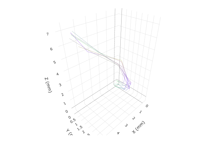
Orientation coloring

Standard DTI color convention: R/G/B = left–right / ant–post / sup–inf

rtists — coloring by diffusion metrics

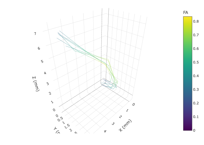
# Color by FA (per-point scalar)
rtists::plot3d(bundle, color = "FA", palette = "Viridis")

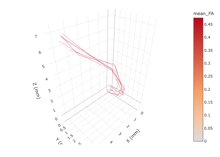
# Uniform color per streamline (mean FA)
rtists::plot3d(bundle, color = "mean_FA", palette = "RdYlBu")

📦 Install: pak::pak("tractoverse/rtists")  |  🔗 tractoverse.github.io/rtists

mascot — reference datasets

Macroscale Structural Connectomes via Tractography (data package)

On-demand download, locally cached.
All datasets returned as fiber::bundle objects.

HCP1065 population atlas (CC BY-SA 4.0)

• 87 white matter bundles
• Averaged across 1,065 healthy HCP adults
• Yeh et al. (2022), Nature Communications

TractSeg per-subject bundles (CC BY-NC 4.0)

• 72 tracts × 105 HCP Young Adult subjects
• Segmented with TractSeg
• Wasserthal et al. (2018), NeuroImage

library(mascot)

# Browse available bundles
available_bundles("HCP1065")
#>  [1] "Anterior Commissure" "Left Arcuate Fasciculus"   ...

# Load by name (downloads once, cached)
cst_left <- HCP1065_CST_L()
cst_left
#> ── Object of class `fiber::bundle()` with 5577 streamliness
#> and [234–291] points per streamline. ──
#>
#> • Point attributes: none
#> • Streamline attributes: none
#> • Bundle attributes: none

# Or the generic importer
bundle <- import_bundle(
  dataset = "TractSeg", 
  bundle = "Left Arcuate Fasciculus", 
  subjects = "599469"
)

mascot — real tractography in a line

library(mascot)
library(rtists)
# Population-average corticospinal tract (left hemisphere)
cst <- HCP1065_CST_L()
# Instantly visualize
plot3d(cst) # orientation RGB