Specialized method to plot mfData objects

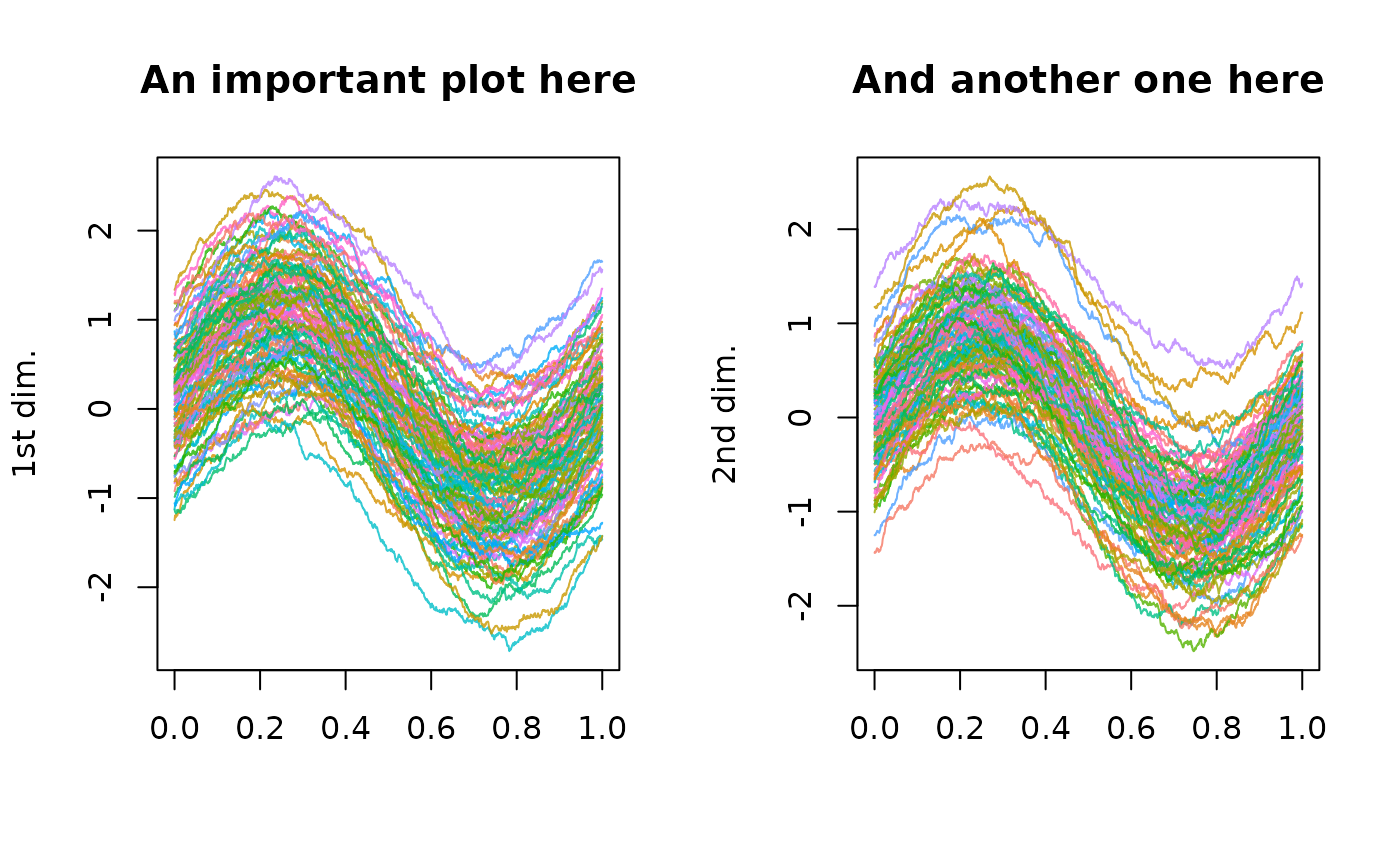
This function performs the plot of a functional multivariate dataset stored in an object of class mfData. It is able to accept all the usual customizable graphical parameters, otherwise it will use the default ones.

# S3 method for mfData
plot(x, ...)

Arguments

x

the multivariate functional dataset in form of mfData object.

...

additional graphical parameters to be used in plotting functions (see Details for the use of ylab and main).

Details

The current active graphical device is split into a number of sub-figures, each one meant to contain the plot of the corresponding dimension of the mfData object. In particular, they are arranged in a rectangular lattice with a number of rows equal to \( \lfloor \sqrt{ L } \rfloor \) and a number of columns equal to \( \lceil L / \lfloor \sqrt{L} \rfloor \rceil \).

A special use of the graphical parameters allows to set up y-labels and titles for all the sub-figures in the graphical window. In particular, parameters ylab and main can take as argument either a single string, that are repeatedly used for all the sub-graphics, or a list of different strings (one for each of the L dimensions) that have to be used in the corresponding graphic.

See also

mfData, fData, plot.fData

Examples

N = 1e2

P = 1e3

t0 = 0
t1 = 1

# Defining the measurement grid
grid = seq( t0, t1, length.out = P )

# Generating an exponential covariance matrix to be used in the simulation of
# the functional datasets (see the related help for details)
C = exp_cov_function( grid, alpha = 0.3, beta = 0.4 )

# Simulating the measurements of two univariate functional datasets with
# required center and covariance function
Data_1 = generate_gauss_fdata( N, centerline = sin( 2 * pi * grid ), Cov = C )
Data_2 = generate_gauss_fdata( N, centerline = sin( 2 * pi * grid ), Cov = C )

# Building the mfData object and plotting tt
plot( mfData( grid, list( Data_1, Data_2 ) ),
      xlab = 'time', ylab = list( '1st dim.', '2nd dim.' ),
      main = list( 'An important plot here', 'And another one here' ) )