Accessing data & building the book

Reproducible Workflows · Session 2

1 Recap: Session 1 → Session 2

1.1 Where we are

Last session you learned the document mechanics; today we fill them with real work.

  • Session 1: write, Quarto documents, structured reports, transparency.
  • Session 2 (today): source, get a real dataset, clean it, version it with git, land your analysis inside the portfolio book, and pick your Chapter-1 dataset.
  • Session 3: publish, pin the environment (uvr), deepen git (PRs, review), put it at a URL, and finish Chapter 1.

Today’s payoff: Chapter 1 (the EDA project) of your portfolio book becomes real. Let’s trace the reproducible data journey end to end.

2 The EDA loop & cleaning decisions

2.1 What EDA is for

Exploratory data analysis (EDA) is the back-and-forth loop where you learn what the data can tell you:

  1. Get a quick sense: shapes, types, missingness, ranges.
  2. Look for problems: wrong types, missing values, inconsistent names/labels, outliers.
  3. Ask & plot: small targeted plots to answer questions and surface surprises.
  4. Record decisions: every cleaning choice documented, because a defensible choice is a feature.

EDA is iterative: you circle through 1–3 several times before any formal modelling. The output that survives into a report is the cleaned data plus the story of your decisions.

2.2 The environment at a glance

Your IDE is part of the reproducible loop. In Positron:

  • Data pane / variable explorer: inspect loaded tables and objects without typing.
  • Inline plots: plots render in the IDE as you iterate.
  • But: the IDE is for exploring; the document is the record. Anything you discover by clicking must end up as code in a .qmd to be reproducible.

Rule: explore by clicking, report by code. The click is fast; the code is what makes it reproducible.

2.3 One-line summaries: skimr::skim()

A whole data set summarized in one call, the fastest honest “first look”:

penguins |> 
  skimr::skim() |> 
  summary()
Data summary
Name penguins
Number of rows 344
Number of columns 8
_______________________
Column type frequency:
factor 3
numeric 5
________________________
Group variables None

skim() shows type, n_missing, and mini-distributions per column in one go (here compacted with |> summary()). When someone asks “what’s in this data?”, skim() first.

2.4 Cleaning names & counting: {janitor}

Real-world data arrives with messy names and labels. {janitor} tidies them:

penguins |>
  janitor::clean_names() |>        # lower-case, underscores, no spaces
  dplyr::slice(1:3) |> 
  gt::gt() |> 
  gt::opt_stylize(style = 4)
penguins |>
  janitor::tabyl(species) |>          # a nicer table() for one variable
  gt::gt() |> 
  gt::opt_stylize(style = 4)

clean_names() makes column names syntactic (safe to reference); tabyl() gives counts with percentages. Both make downstream code far more readable.

2.5 Diagnosing missingness: skim + naniar

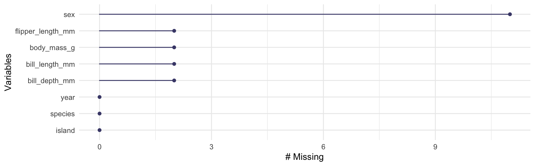
Before choosing what to do, first see where and how much data is missing. {skimr} (a few slides ago) reports n_missing per column; {naniar} turns missingness into a figure with legible per-column counts, as in Figure 1:

naniar::gg_miss_var(penguins)
Figure 1: How much is missing per column, at a glance.

gg_miss_var() plots the number of missing values per column with horizontal, readable labels; vis_miss() grids the data set to show the pattern case by case. naniar’s site lists many more missingness helpers.

2.6 Dealing with missing values

Once you’ve diagnosed it, decide how to handle it. Three honest strategies; each is a documented decision, not a default:

  1. Drop with tidyr::drop_na(): simplest, but you may lose whole columns or many rows; only acceptable when the missing cases are few and not systematically different.
  2. Impute (fill in a plausible value): keeps all cases, but imputed values are estimated, not observed. The MissingData CRAN Task View is the curated map of R’s methods.
  3. Keep and use na.rm = TRUE: let functions skip NA where they support it; cheapest when missingness is sparse and local.

No free lunch: dropping loses information, imputing adds an assumption, na.rm = TRUE only defers the decision. Diagnose first (skim + naniar), then choose and write down why. Where you can, make that call together with the domain experts who know what each NA actually means in this data.

2.7 Tying it to Session 1

This is the same cleaning conversation you started in the base-R course with penguins_messy.txt:

  • There you fixed wrong types (readr guessing), separators, and missing values by hand.
  • Today the decisions are the point: janitor, naniar, skimr don’t make them for you; they surface them faster so you can decide well and record why.

The toolkit changed; the habit didn’t: inspect → decide → document. Every decision you can justify in a sentence is a reproducible decision.

2.8 Your turn: EDA toolkit

Run this on the penguins data (loaded at the top), or a data frame of your own:

  1. skim(penguins): which columns have missing values? How many?
  2. penguins |> clean_names() |> names(): do names need cleaning?
  3. penguins |> tabyl(species): what are the group sizes?
  4. penguins |> tabyl(species) |> gt::gt() |> gt::opt_stylize(style = 4): present those counts as a styled table (the {gt} you met in Session 1).
  5. vis_miss(penguins): where is the missingness concentrated?
  6. Write one sentence: “I will handle the missingness by … because …”, that sentence is your reproducible cleaning decision.

3 Sourcing open data

3.1 Open data, anywhere in the world

A reproducible analysis needs data it can re-fetch by code, and open-data portals everywhere provide exactly that:

  • France: data.gouv.fr, thousands of public datasets, license-aware.
  • Your own country: nearly every government runs an official open-data portal (data.gov… for the US, Canada, UK, Germany, and many more).
  • The rule is the same wherever you look: a dataset you can fetch programmatically is a dataset your analysis can re-produce.

The reproducible move: don’t download a dataset by hand; write code that sources it, so the analysis is re-runnable and the provenance (publisher + URL) is in the document.

3.2 {rdatagouv}: the French portal from R (an option)

Because we teach from l’ENSAI, data.gouv.fr is a natural default. Its thousands of public datasets trend toward the public, transport, environment and culture topics the French job market cares about, and they’re license-aware, so the dataset you showcase is safe to publish. {rdatagouv} (maintained by your instructor) wraps it:

Why a natural pick: pick a topic you care about that a future recruiter would also find compelling once your portfolio is online. Whatever you choose, {rdatagouv} is an option, not a requirement: any portal you can query with a URL (e.g. download.file()) works just as well for reproducibility.

3.3 Fetching any portal by URL

Whatever portal you choose, the reproducible core is the same: a URL your code downloads:

  • download.file() is portal-agnostic: it doesn’t care whether the URL points at data.gouv.fr or your home country’s portal.
  • Pair it with a provenance sentence (dataset, publisher, URL, license) so a reader can find and trust the source.
  • Some portals ship an R/Python client ({rdatagouv} here): a convenience, never a requirement.

Live block (≈10 min). Together: rdatagouv::dg_find_datasets(q = "climat", schema_only = TRUE) and browse one non-French portal (e.g. your home country’s). Both approaches collapse to the same thing: a URL to download by code.

3.4 Data that ships as an R package

Not every dataset needs a portal: many ship inside an R (or Python) package, and that’s reproducible too. You’ve used one already, palmerpenguins::penguins.

  • A versioned package is reproducible data: the package is properly released and versioned on CRAN (or PyPI), and its docs and provenance ship with it.
  • Because it’s a package, your environment manager (uvr/uv) can lock its exact version, so a re-render gets the same data today and next year.
  • Good examples: {gapminder}, {nycflights13}, {babynames}, {Lahman} (baseball), {tidycensus}, {rdatagouv}’s returned data.

A packaged dataset is the ultimate reproducible source: one line to load, an immutable version, documented. That’s why today’s analysis can trust palmerpenguins without a portal or a download.file().

3.5 Finding data by code: catalogues & portal APIs

Beyond your default portal, two more reproducible ways to find a dataset by code:

  • Curated catalogues of packaged data: the Rdatasets list indexes hundreds of datasets shipping in CRAN packages, each loadable in one line; browse the CRAN package list and search by name.
  • Portal-API packages, one wrapper per portal, same convenience as {rdatagouv}: {ausOpenData}, {opendatatoronto}, {SeattleOpenData}, {sfOpenData}, {laOpenData}, {chiOpenData}, {nycOpenData}, {nysOpenData}, {nolaOpenData}, {mtaOpenData}, {cincinattiOpenData}, {ColOpenData}, {ctOpenData}, {deOpenData}, {istat}, {istatR}, {COVID19}.

Every route collapses to the same reproducible core: a packaged dataset (versioned with its package) or a portal you query by code, both with provenance you can record. The portal is optional; the code you can re-run is not.

3.6 Lab 1: your dataset

Lab 1 (≈35 min): lab-1-eda-datagouv.qmd.

  1. Pick a dataset you actually care about, from any source we’ve covered: an open-data portal (via {rdatagouv}, a portal-API package, or download.file()), or a dataset that ships in a package (e.g. from the Rdatasets catalogue).
  2. In a Quarto doc, source it by code (no manual download), {rdatagouv} for data.gouv, download.file() for any portal, the package call for a packaged dataset.
  3. Run a quick EDA: skim(), clean_names(), tabyl(), vis_miss().
  4. Write 2–3 sentences on your cleaning decisions.

4 Versioning your data with {pins}

4.1 The (dis)appearing data problem

Last session you met “the (dis)appearing data”: a fetched file can change or vanish the moment it’s off the portal:

  • A portal updates a dataset: your analysis was based on the old version.
  • A raw URL 404s a year later, and your “reproducible” document can’t re-run.
  • Even locally, data/my-data.csv can be overwritten, and git alone doesn’t version the cached copy well if you don’t commit it.

{pins} closes that gap: version your data the way git versions your code, so a re-render gets the same data a reader expects, not whatever is live today.

4.2 {pins}: pin data to a versioned board

{pins} stores a data object on a board and records who wrote what, when:

# a folder board that KEEPS HISTORY (versioned = TRUE)
bd <- pins::board_folder(path = "pins/", versioned = TRUE)

# fetch open data once, then pin it:
dat <- readr::read_csv("https://…/my-open-dataset.csv")
pins::pin_write(board = bd, x = dat, name = "my-dataset")        # snapshot it, versioned & hashed

# later re-reads get the PINNED copy, reproducibly:
pins::pin_read(board = bd, name = "my-dataset")

pin_write() snapshots the data and records the version + hash; pin_read() returns that exact snapshot. Re-render → same data, every time.

4.3 Where the versioned copy lives

A board is just a folder (or a service), and it’s fully inspectable:

  • pin_list(board): what’s been pinned.
  • pin_versions(board, "my-dataset"): every snapshot, with hashes and dates.
  • pin_read(board, "my-dataset", version = "…"): roll back to an older snapshot.

The pinned pins/ folder is committed alongside your code, so the exact data your analysis used is reproducible forever, independent of portal changes or broken URLs.

4.4 Fetch once, pin, analyse

A reproducible data workflow in three deliberate steps:

  1. Fetch the open data by URL: provenance recorded.
  2. Pin it with pin_write(): versioned & hashed on a local board.
  3. Analyse from the pinned copy (pin_read()): stable no matter what happens upstream.

Pinning keeps you honest: the data you analysed is on record, not just the code. Combined with git (code), uvr/uv (environment) and a URL (delivery), it completes the durable portfolio you build in Session 3.

4.5 Beyond data: version your models too

The same “pin what you made” idea extends to the models you fit, not just the data:

  • {vetiver}: pins a model to a board, so the exact trained model is deployed or re-loaded, versioned & reproducible like your data.
  • It pairs with pin_write()/pin_read(): you already know the mechanics; {vetiver} just knows how to save/load a model’s metadata too.

Same habit, new object

data → {pins}, model → {vetiver}, code → git/GitHub

Saving a trained model by hand usually loses which packages/versions made it. {vetiver} records those alongside the model, so it re-runs and re-deploys anywhere.

4.6 R and Python, side by side

Every reproducibility tool you’ve met has an equivalent in Python, with the same ideas and the same names:

Role R Python
Environment uvr uv
Data & artifacts {pins} {pins}
Model versioning/deploy {vetiver} {vetiver}

Your book is Python-compatible by design: whichever language a chapter uses, the reproducible pipeline (source → pin → version → publish) is the same. Only the environment row is a preview: you’ll actually pin it (uvr/uv) in Session 3, once the whole data-to-publish loop is in place.

5 Versioning your code with git

5.1 Git in one habit

You version your data with {pins}; you version your code with git, one round at a time:

git status             # your compass: where am I?
git add <file>        # stage the changes you want to keep
git commit -m "msg"   # snapshot with a note
git push              # send the snapshot to GitHub
  • usethis::use_git() turns the folder into a git repo; the Positron git pane is the clickable version of the loop.
  • Commit often: small, descriptive commits beat rare mega-commits; git status is your compass.

Version your code the way you just versioned your data. add → commit → push is the whole habit; everything else is dress-up.

5.2 A repo + a remote

Local history is half the story; a remote (GitHub) makes it durable and shareable:

usethis::use_git()        # make it a git repo
usethis::use_github()     # create + link the remote, push once
  • Set up a GitHub account first, then register a PAT with gitcreds::gitcreds_set() (mini-lab below); without it, Positron pushes can’t authenticate.
  • {usethis} runs it all: use_git() to init, use_github() to link the remote and push once.
  • In the Positron git pane, the push button sends your commits to GitHub.

A pushed repo is a backup and a way to share; a local-only repo is one laptop failure from gone. Push early, push often.

5.3 .gitignore: what NOT to commit

Not everything belongs in history. Tell git to ignore machine-local noise:

cat .gitignore
  • R: .Rhistory, .RData, renv/library/
  • Render output: _book/, *_files/
  • Editor/OS: .DS_Store, .venv/, __pycache__/

Your portfolio-book/.gitignore scaffold already covers these. The rule: commit source, not output or environment. Source is what rebuilds everything.

5.4 Branches: keep main always-working

A branch is a second history you can work on without touching main:

git checkout -b eda-chapter-1          # make + switch to a branch
# work on it
git commit -am "add chapter 1"         # stage + snapshot
git push -u origin eda-chapter-1       # share the branch early
# each time you re-work it, re-align with main:
git checkout main && git fetch --all --prune && git pull
git checkout eda-chapter-1 && git merge main
  • Mirror how you actually work: try an idea on a branch, keep it if it works; main stays always-working.
  • In the Positron git pane, the branch menu creates and switches branches.

Re-align with main often so conflicts stay small; never push to main directly (Session 3’s pull request decides what merges).

5.5 Connect with your instructor

Mini-lab (~10 min). Get your book onto GitHub to share and get feedback during the gap week:

  1. If you haven’t yet, create and store a PAT: usethis::create_github_token() then gitcreds::gitcreds_set().
  2. usethis::use_git() then use_github() on your portfolio book.
  3. Make a real change, commit, push (git add / git commit / git push).
  4. Branch git checkout -b eda-chapter-1, push it too.

By the end of today, your book is versioned, remote, and ready to review.

6 Quarto books

6.1 What a Quarto book is

A book bundles many .qmd chapters into one navigable publication:

  • project: type: book marks the folder; _quarto.yml lists chapters in order.
  • Each .qmd is a chapter; they cross-reference and share figures/tables.
  • Render once → a site with sidebar navigation, TOC, bibliography.

You already know the document mechanics: a book is the same thing scaled to many files, wired together in _quarto.yml.

6.2 Anatomy of _quarto.yml

The book is driven by one small file:

project:
  type: book
book:
  title: "My Data Science Portfolio"
  author: "Your Name"
  chapters:
    - index.qmd
    - chapters/01-EDA.qmd
    - references.qmd
bibliography: references.bib
format:
  html:
    theme: cosmo

Add a chapter by appending its path to chapters:; list order is book order.

6.3 Make it yours: branding

The book’s look is yours to define. Two files beside _quarto.yml control it:

# colours & fonts (the zero-CSS on-ramp)
color:
  palette:
    teal:   "#2E7D6B"   # pick your own accents
    amber:  "#E8A33D"
    indigo: "#4A5899"
    ink:    "#17251F"
    paper:  "#F1EEE6"
  primary: teal
  foreground: ink
  background: paper
/* structural CSS beyond the palette */
/* find selectors via Inspect, then tweak */
.sidebar { width: 300px; }

Edit a "#hex", quarto preview, look. Match what you like, not the course decks.

6.4 Language-agnostic chapters

A Quarto book happily mixes languages, and so can your portfolio:

  • Chapter files are just .qmd; each chapter can run R, Python, or both.
  • format: html and cross-references work identically either way.
  • That’s why your portfolio stays useful as you grow into Python in later courses.

Portfolio-first design: the scaffold already reserves empty chapters for later instructors (02-semester-2.qmd, 03-semester-3.qmd). Your book is built to grow.

6.5 Lab 2: build your book

Lab 2 (≈35 min): lab-2-portfolio-book.qmd.

  1. Download the starter book: grab portfolio-book.zip from the course materials page (https://astamm.github.io/r-ensai/reproducible-workflows/#materials) and unzip it.
  2. Render it: confirm the starter book builds.
  3. Drop your Lab-1 EDA in as Chapter 1 (chapters/01-EDA.qmd).
  4. Re-render the whole book; check the sidebar and cross-references.

7 Finding a great dataset

7.1 Beyond data.gouv.fr: OpenData R packages

Pick the portal (or package) that gets you to a dataset you care about; the reproducibility rule never changes:

  • France: data.gouv.fr via {rdatagouv}.
  • Your country: nearly every government runs an official portal (data.gov for the US, Canada, UK, Germany…), fetched by URL.
  • R-friendly datasets: {tidycensus} (US Census), {opendatatoronto}, #TidyTuesday data on GitHub; Kaggle datasets too.

Whatever the source, the bar is the same: you can fetch it by code and record its provenance (dataset, publisher, URL, license). If you can download it with one line of code, it’s fair game for Chapter 1.

7.2 Choose your dataset before you leave

Final task of the session (~10 min). Leave today having chosen your Chapter-1 dataset so Session 3’s work block starts fast:

  1. Pick a dataset you actually care about on data.gouv.fr, your country’s portal, or an R-friendly source above.
  2. Record its source by code (a URL / a package call) and its provenance (publisher, URL, license).
  3. Write one line: the question you want to answer with it. That question is your IMRAD seed for Chapter 1.

8 Writing for an audience

8.1 A report is read, not just rendered

Your EDA will be read by other humans, instructors, classmates, future employers. Write to them:

  1. Structure signals intent: question, data, cleaning, results, findings.
  2. Captions do the explaining: a reader should grasp a figure from its caption before reading your prose.
  3. Say what you found and what you didn’t: honest limits are credibility.
  4. Keep code in service of the story: the code shows how; the prose says why it matters.

The reproducibility narrative: because everything is code and captioned, a stranger re-rendering your .qmd both trusts and reproduces your work. That’s the product.

8.2 Preparing work others will extend

Your chapters are slots other courses will fill. Make that easy:

  • Use the same structure every time (the 5-section recipe).
  • Give descriptive labels to figures/tables (fig-cap everywhere).
  • Keep setup in one chunk so new chapters start from a known environment.
  • Leave placeholder chapters in place: they’re the roadmap.

Think of the book as a shared, growing artefact, not a one-off. Every convention you follow today lowers the friction for the next instructor who appends a chapter.

8.3 Recap: the full loop

From data to a readable, reproducible chapter, the whole course in one picture:

  1. Source open data by code (portal of your choice): provenance recorded.
  2. Explore & clean ({skimr}/{janitor}/{naniar}): decisions documented.
  3. Report in a structured chapter: captions, cross-refs, findings.
  4. Assemble into the book: one navigable portfolio.
  5. Version your work on git: committed, branched, pushed to GitHub (today).
  6. (Session 3) Pin & publish: uvr/uv ({pins} for data), Posit Connect.

Today you’ve done steps 1–5: your book is sourced, cleaned, assembled, and under version control. Step 6 (Session 3) pins the environment, reviews through a PR, and turns the local book into a shared, durable URL.

8.4 Three moves, one book

Source, clean, build.

8.5 Source, clean, build

Today your book gained its first real chapter.

Source by code

Open data fetched by code (any portal) and pinned with {pins}: provenance (publisher + URL) recorded.

Clean with evidence

skimr/janitor/naniar: decisions documented as why, not just what, so a stranger can trust them.

Build Chapter 1

Your EDA assembled into the book: captioned, cross-referenced, written for a reader.

8.6 Your Chapter 1, committed

From a local chapter to a durable, shareable book.

Build Chapter 1: make it durable next

Everything today lives in 01-EDA.qmd inside your book, versioned on git and pushed to GitHub. In Session 3 that chapter becomes published: uvr/uv pins its environment and R version (and today’s {pins} board versions its data), it’s reviewed through a pull request, then Posit Connect gives it a URL. Same book, suddenly a published, reproducible portfolio.

8.7 Next time

Session 3: version it, pin it, publish it.

Between sessions: finish lab-2-portfolio-book.qmd so your book builds, commit it to GitHub on your eda-chapter-1 branch, and refine your Chapter 1 dataset and question. Your instructor can already comment on it there; bring it ready to publish next session.